Analysing clades and traits in a metacommunity

This article goes through the two analyses of metacommunity phylogenetics in the package: the node regression of Leibold et al. (2010) with their daphniids, and the phylogenetic gradient analysis of Peres-Neto et al. (2012) with simulated data, which are the methods checked in the article on validation.

library(comdynamite)

Which clades respond to the environment?

daphniids rebuilds the data of Leibold et al. (2010) from the public survey: presences of 13 species in lakes of the northeastern United States, nine predictors and six biogeographic contrasts. node_contrasts() codes each node of the tree as a contrast between its two clades. This tree has no branch lengths; with them, branch_lengths = TRUE gives the coding of the supplement of the article.

nodes <- node_contrasts(daphniids$tree)
dim(nodes)
#> [1] 13 12

node_test() regresses each contrast on the predictors. The default of 9999 permutations suits the false discovery rate. We use 999 here to keep the page quick to build, with nodes in parallel on two cores.

set.seed(1)
out <- node_test(daphniids$comm, nodes, daphniids$env, daphniids$biogeography, n_perm = 999,
                 cores = 2)
out
#> <mc_node_test> 12 nodes, 11 tested
#> permutations: 999 free of sites, 999 of species; smallest possible p: 0.001 
#> nodes with p (max) <= 0.05: 0 before correction, 0 after
#> nodes not tested: 1 (a clade without individuals, too few sites or a predictor without variance in the sites of the node)

The p-values answer different questions, so this choice comes first. p_max tests the association between predictors and phylogeny, and it needs both permutations to reject. With 13 species, permutations of species have little power, so nothing passes it here. Permuting sites alone tests whether a predictor matters for that contrast, whether or not that comes from phylogeny. The figures below use sites, as this recovers most of the results of the article, and should be read with that limit in mind.

plot_node_test() places the results on the tree, as in Figure 3 of the article.

plot_node_test(out, daphniids$tree, test = "site")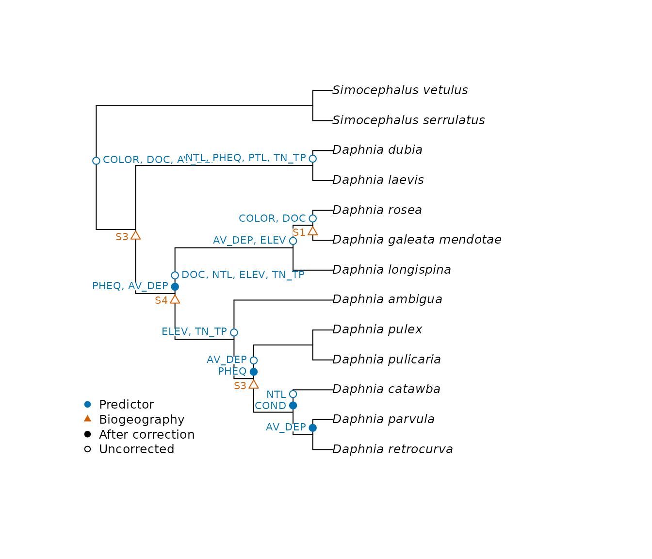

A tree of this size reads best as a phylogram. For very large trees, type = "fan" draws the same plot in less space.

plot_node_heatmap() gives the direction and size of each association, as in Table S1 of the article.

plot_node_heatmap(out, test = "site")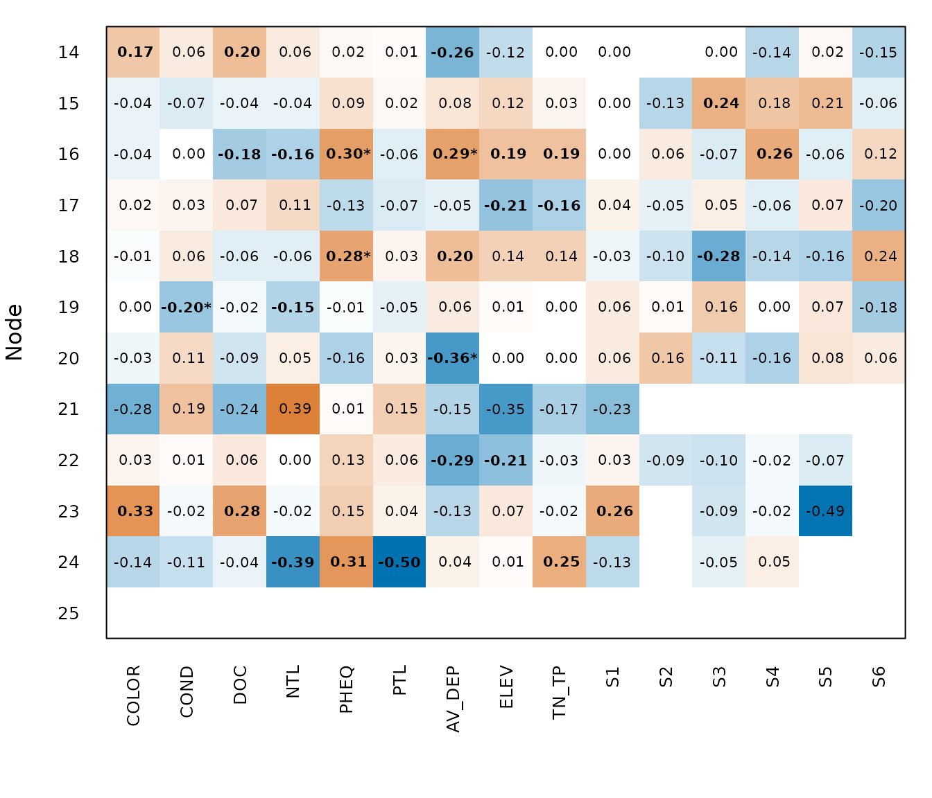

A positive value means that the second clade of the node, in the order of the tree, is favoured where the predictor is high.

Coding biogeographic events

biogeography_matrix() builds the events from the area of each site. Events should come from a hypothesis stated in advance, as the areas on the two sides of a barrier (Leibold et al. 2010; Leibold & Chase 2018). Here, three regions are separated by two barriers, and the later one splits the last two regions.

region <- rep(c("north", "centre", "south", NA), c(8, 6, 6, 10))
events <- list(barrier = list("north", c("centre", "south")),
               river = list("centre", "south"))
head(biogeography_matrix(region, events, min_sites = 3))
#>      barrier river
#> [1,]       1     0
#> [2,]       1     0
#> [3,]       1     0
#> [4,]       1     0
#> [5,]       1     0
#> [6,]       1     0

contrast = "others" compares each area with the rest, for example each refugium with the other refugia. It needs no hypothesis about how areas relate, so it asks a weaker question.

Sites of an area are often neighbours, and free permutations then reject too often. We simulated 1000 metacommunities on a torus of 15 by 15 sites, with communities that followed a hidden autocorrelated environment and two blocks of 25 sites placed at random, so that events had no effect (data-raw/validation_events.R). Free permutations rejected 45.1% of the tests of a node at the 5% level, and permutations from torus_permutations(), given in site_permutations, rejected 4.8%. The events in the figures above used free permutations, so they should be read with this in mind. Landscapes with edges need a restricted null model chosen for them, and a matrix of permutations of any origin can be given.

How much of the phylogenetic structure is due to environment and space?

For this question we need a tree with branch lengths and sites with coordinates, so we simulate them with the generator of Appendix C of Peres-Neto et al. (2012). In the first scenario, two independent gradients act on species.

set.seed(1)
tree <- treeshapesim::sim_tree_shape(32, beta = 10)
gradients <- logistic_gradients(1)
sim <- simulate_logistic(tree, gradients[c("x", "y")])
keep <- rowSums(sim$abundance) > 0
comm <- sim$abundance[keep, ]
comm <- comm[, colSums(comm) > 0]
x <- gradients$x[keep]
y <- gradients$y[keep]

A high beta gives a balanced tree, as in that appendix. phylo_vector() tests whether a gradient is related to the phylogeny and, if so, gives a vector of species values for the next step. Here we ask this for each gradient.

first <- phylo_vector(comm, tree, x, n_perm = 199)
second <- phylo_vector(comm, tree, y, n_perm = 199)
c(first$p_max, second$p_max)
#> [1] 0.005 0.010

trait_partition() then splits the variation of these vectors among sites. The vectors are chosen to fit the gradients, so this step only makes sense after a significant global test.

vectors <- cbind(first$pev_brown, second$pev_brown)
partition <- trait_partition(comm, vectors, x, y, n_perm = 199)
partition
#> <mc_trait_partition> mean component, 0.559 of the total variation
#> permutations: 199 free of sites, 199 of species; smallest possible p: 0.005 
#>   fraction     r2 r2_adjusted r2_component p_site p_taxa p_max
#> 1      abc 0.4392      0.3991        0.785  0.005  0.005 0.005
#> 2       ab 0.2613      0.2358        0.467  0.005  0.005 0.005
#> 3       bc 0.2607      0.2352        0.466  0.005  0.005 0.005
#> 4        a 0.1784      0.1639        0.319  0.005  0.005 0.005
#> 5        b 0.0828      0.0719        0.148     NA     NA    NA
#> 6        c 0.1779      0.1633        0.318  0.005  0.005 0.005
#> 7        d 0.5608      0.6009        0.215     NA     NA    NA
round(partition$semipartial, 2)
#>        trait1 trait2
#> env1     0.52  -0.29
#> space1  -0.24   0.55

plot_trait_partition(partition, labels = c("Gradient x", "Gradient y"))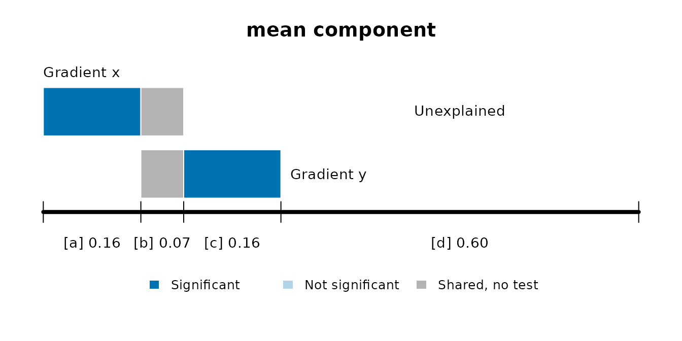

The test of each trait against each predictor is a different question, for which ter Braak (2019) is the reference.

References

Leibold, M. A., & Chase, J. M. (2018). Metacommunity Ecology. Monographs in Population Biology 59. Princeton University Press. https://doi.org/10.2307/j.ctt1wf4d24

Leibold, M. A., Economo, E. P., & Peres-Neto, P. (2010). Metacommunity phylogenetics: separating the roles of environmental filters and historical biogeography. Ecology Letters, 13, 1290–1299. https://doi.org/10.1111/j.1461-0248.2010.01523.x

Peres-Neto, P. R., Leibold, M. A., & Dray, S. (2012). Assessing the effects of spatial contingency and environmental filtering on metacommunity phylogenetics. Ecology, 93, S14–S30. https://doi.org/10.1890/11-0494.1

ter Braak, C. J. F. (2019). New robust weighted averaging- and model-based methods for assessing trait-environment relationships. Methods in Ecology and Evolution, 10, 1962–1971. https://doi.org/10.1111/2041-210X.13278