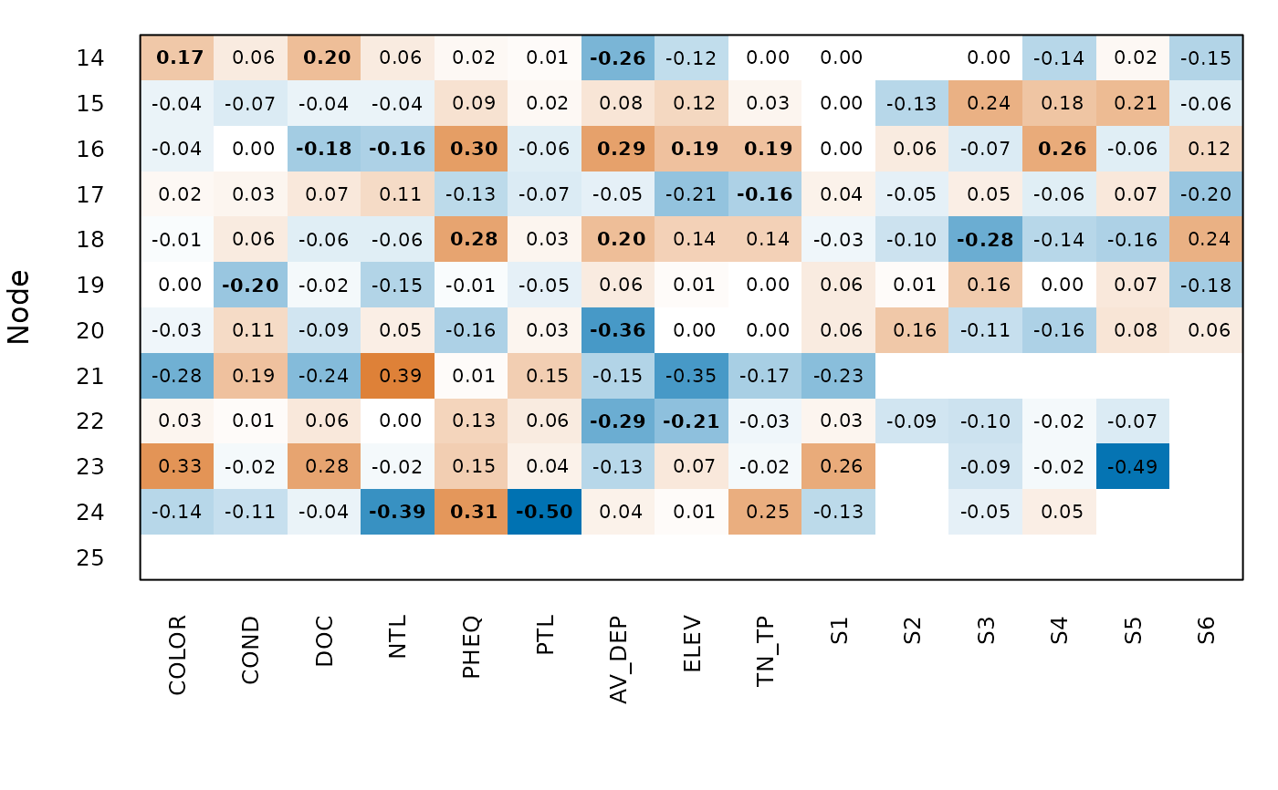
Plot the semipartial correlations of a node test — plot_node

Draws a table of nodes by variables with the semipartial correlations of node_test(), as in Table S1 of Leibold et al. (2010). Bold values with an asterisk remain significant after the false discovery rate, as in plot_node_test(); other bold values are significant only as isolated tests. Blank cells could not be calculated.

Usage

plot_node_heatmap(
  x,
  test = c("max", "site", "joint"),
  alpha = 0.05,
  col = c("#0072B2", "#D55E00"),
  cex = 0.8,
  ...
)

Arguments

x: Result of node_test().
test: Permutation test to show: "max" for the larger p-value of sites and species, "site" for sites alone, or "joint" for the permutation of the article. See node_test() for what each one tests.
alpha: Significance level.
col: Colours of negative and positive values.
cex: Size of the text.
...: Other arguments of graphics::image().

Value

Invisibly, the matrix of semipartial correlations, with predictors followed by biogeographic events.

Details

Rows are the node numbers of the tree. To find them, call ape::nodelabels() after plot_node_test().

References

Leibold, M. A., Economo, E. P., & Peres-Neto, P. (2010). Metacommunity phylogenetics: separating the roles of environmental filters and historical biogeography. Ecology Letters, 13, 1290–1299. doi:10.1111/j.1461-0248.2010.01523.x

Examples

nodes <- node_contrasts(daphniids$tree)
set.seed(1)
out <- node_test(daphniids$comm, nodes, daphniids$env, daphniids$biogeography,
                 n_perm = 49)
plot_node_heatmap(out, test = "site")