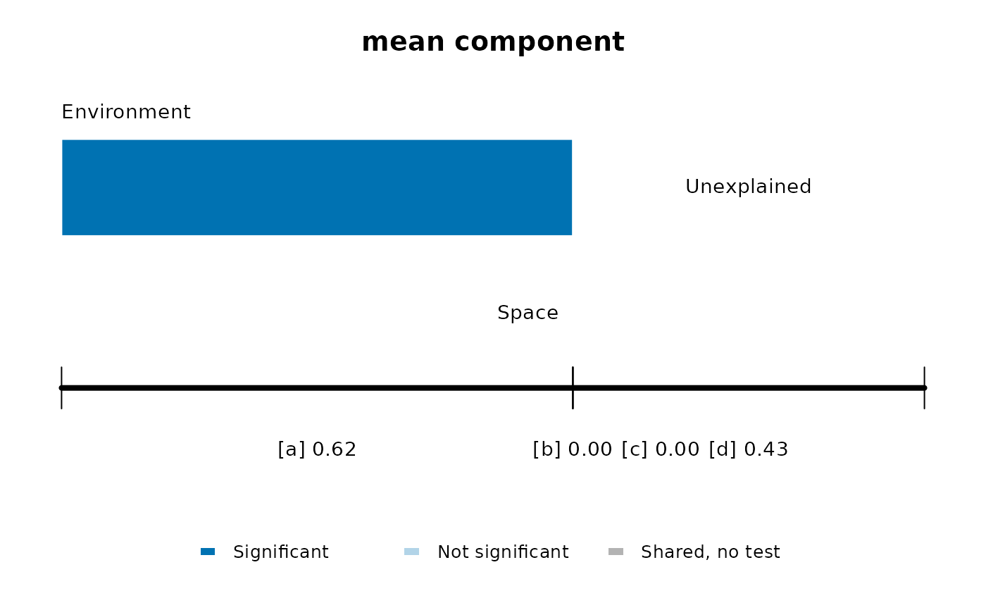
Plot the fractions of a trait partition — plot_trait

Draws the total variation as a line divided into the fractions of trait_partition(), with one bar for the environment and one for space, as in Figure 1 of Desdevises et al. (2003). The two bars overlap in b, the variation they share. a is explained by the environment alone, c by space alone, and d is unexplained. Dark segments are significant, and b has no test, so it is grey.

Usage

plot_trait_partition(
  x,
  value = c("r2_adjusted", "r2", "r2_component"),
  test = c("max", "site", "taxa"),
  alpha = 0.05,
  col = "#0072B2",
  labels = c("Environment", "Space"),
  cex = 0.9,
  ...
)

Arguments

x: Result of trait_partition().
value: Column of the fractions to show: "r2_adjusted", "r2", or "r2_component" for the share of the mean or variance component.
test: Permutation test: "max" for the larger p-value of sites and species, "site" or "taxa".
alpha: Significance level.
col: Colour of significant segments.
labels: Names of the two sets of predictors.
cex: Size of the text.
...: Other arguments of graphics::plot.window().

Value

Invisibly, the rows of x$fractions for a, b, c and d, with shown, the values drawn.

Details

Negative fractions are shown as zero, following Legendre (2008). The result of trait_partition() keeps them, because all fractions sum to one only with them.

References

Desdevises, Y., Legendre, P., Azouzi, L., & Morand, S. (2003). Quantifying phylogenetically structured environmental variation. Evolution, 57, 2647–2652. doi:10.1111/j.0014-3820.2003.tb01508.x

Legendre, P. (2008). Studying beta diversity: ecological variation partitioning by multiple regression and canonical analysis. Journal of Plant Ecology, 1, 3–8. doi:10.1093/jpe/rtm001

Examples

set.seed(1)
trait <- stats::setNames(seq(0, 100, 10), letters[1:11])
env <- runif(40, 0, 100)
space <- cbind(runif(40), runif(40))
comm <- outer(env, trait, function(e, t) exp(-(e - t)^2 / 800))
colnames(comm) <- names(trait)
out <- trait_partition(comm, trait, env, space, n_perm = 49)
plot_trait_partition(out)