Evaluating a method with simulated metacommunities • comdynamite

A statistical method for community data should be evaluated on data where the truth is known. Simulations give that truth: they let us measure how often a test rejects a null hypothesis that is true (type I error) and how often it rejects one that is false (power). This vignette shows the workflow with a simple question: does a permutation test of the association between community composition and a predictor keep its nominal error rate in a spatially structured metacommunity?

The simulations take a few minutes, so the results were computed in advance and are loaded below. The complete script is data-raw/vignette_method.R. The same steps apply to any other method: replace the function in step 2.

Step 1: simulate data with a known truth

We simulate metacommunities on a 10 x 10 torus with an autocorrelated environment and limited dispersal. Besides the environment that drives the community, we draw a second predictor with the same autocorrelation but no relation to the community. Testing the true environment measures power; testing the unrelated predictor measures the type I error.

library(comdynamite)
side <- 10
tree <- treeshapesim::sim_tree_shape(30)
land <- landscape_grid(side, env_bandwidth = 2, disp_scale = 2)
unrelated <- landscape_grid(side, env_bandwidth = 2)$env

traits <- species_traits(tree, lambda = 1, sigma_mean = 8, sigma_sd = 2)
alpha <- competition_matrix(tree, "none")
sim <- simulate_metacommunity(land, traits, alpha, dispersal = 0.05, n_steps = 500)

Keeping the tree and landscape fixed across scenarios within a replicate pairs the comparisons, as here for lambda = 0 and lambda = 1.

Step 2: write the method as a function

The method under evaluation is the proportion of variation in Hellinger- transformed abundances (Legendre & Gallagher 2001) explained by one predictor, as in a redundancy analysis, with a permutation test.

r2_env <- function(y, x) {
  y <- scale(y, scale = FALSE)
  x <- x - mean(x)
  sum((crossprod(x, y) / sum(x^2))^2) * sum(x^2) / sum(y^2)
}
p_value <- function(y, x, perms) {
  obs <- r2_env(y, x)
  null <- apply(perms, 1, function(p) r2_env(y, x[p]))
  (sum(null >= obs) + 1) / (length(null) + 1)
}

Step 3: define the alternatives to compare

We compare two null models. Free permutations treat sites as exchangeable. torus_permutations() keeps the distances among sites, and thus the autocorrelation of the predictor.

n_perm <- 199
free <- t(replicate(n_perm, sample(side^2)))
torus <- torus_permutations(side)
restricted <- torus[sample(nrow(torus), n_perm), ]

y <- vegan::decostand(sim$abundance[, colSums(sim$abundance) > 0], "hellinger")
p_value(y, unrelated, free)
p_value(y, unrelated, restricted)

Step 4: replicate and summarise

Repeating steps 1 to 3 gives one p-value per replicate and scenario. The rejection rate at the 5% level estimates the type I error for the unrelated predictor and the power for the true environment. With 200 replicates, the standard error of a rate near 0.05 is about 0.015.

results <- readRDS("evaluating-methods.rds")
rates <- aggregate(p ~ predictor + null_model + lambda, data = results,
                   FUN = function(p) mean(p <= 0.05))
names(rates)[names(rates) == "p"] <- "rejection_rate"
rates$se <- sqrt(rates$rejection_rate * (1 - rates$rejection_rate) / 200)
knitr::kable(rates, digits = 3)

predictor	null_model	lambda	rejection_rate	se
environment	free	0	1.00	0.000
unrelated	free	0	0.76	0.030
environment	torus	0	1.00	0.000
unrelated	torus	0	0.08	0.019
environment	free	1	1.00	0.000
unrelated	free	1	0.74	0.031
environment	torus	1	1.00	0.000
unrelated	torus	1	0.07	0.018

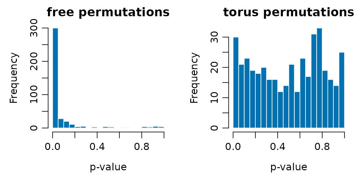
Under a true null hypothesis, p-values should be uniform:

h <- results[results$predictor == "unrelated", ]
old <- par(mfrow = c(1, 2), mar = c(4, 4, 2, 1), mgp = c(2.4, 0.7, 0))
for (n in c("free", "torus")) {
  hist(h$p[h$null_model == n], breaks = seq(0, 1, 0.05), col = "#0072B2",
       border = "white", main = paste(n, "permutations"), xlab = "p-value")
}

Histograms of p-values for the unrelated predictor under free and torus permutations.

par(old)

What the evaluation shows

Free permutations are not valid here. They reject a true null hypothesis in about 75% of replicates, 15 times the nominal rate. Both the community and the unrelated predictor are spatially autocorrelated, so they tend to match by chance, and permuting sites freely breaks this structure in the null distribution but not in the observed statistic (Legendre 1993).

Torus permutations come close to the nominal level. Their rejection rates (0.08 and 0.07) are about two standard errors above 5%, and their p-values are much closer to uniform. More replicates would be needed to tell whether this small excess is real.

This setting does not discriminate power. Both null models reject the true environment in all replicates, because the effect is strong. Power cannot be compared here, and it would not be meaningful for free permutations, whose error rate is not controlled. A study of power would need weaker effects, for example broader niches, higher dispersal or fewer sites.

The phylogenetic signal makes no difference to this test, as expected, because the statistic does not use the tree. The lambda factor is included to show how scenarios enter the design. It would matter for a method that uses phylogenetic information.

Adapting the workflow

Replace r2_env() with your statistic, and the predictors with the hypotheses of your method.
Add scenarios by varying dispersal, niche breadth or the type of competition, and report the rejection rate for each.
Set the number of replicates from the precision you need: the standard error of a rejection rate p is sqrt(p * (1 - p) / n_rep).
Check that the simulated communities are realistic for your question, for example in local richness and occupancy, before interpreting rejection rates.

Tree shape as a factor of the design

The results above use trees from treeshapesim::sim_tree_shape() with its default shape, and the statistic ignores the tree, so tree shape cannot affect them. For a method that uses phylogenetic information, tree shape should be part of the design. The treeshapesim package simulates trees in which imbalance (beta) and branching times (c) are set separately.

set.seed(1)
shapes <- expand.grid(beta = c(-1, 0), c = c(-0.5, 0))
measured <- t(mapply(function(beta, c) {
  trees <- treeshapesim::sim_tree_shape(30, beta = beta, c = c, nsim = 100)
  rowMeans(sapply(trees, treeshapesim::tree_shape))
}, shapes$beta, shapes$c))
knitr::kable(cbind(shapes, measured), digits = 2)

beta	c	gamma	colless
-1	-0.5	-1.61	1.40
0	-0.5	-1.58	-0.02
-1	0.0	0.00	1.22
0	0.0	-0.01	0.14

The table gives the mean gamma statistic and normalized Colless index of 100 trees for each combination. Each tree is a phylo object, so it replaces the tree in step 1 without other changes. To aim at given values of gamma and Colless, use shape_grid() and sim_tree_target() from the same package. The treeshapesim article on comdynamite shows the two packages together.

torus_permutations() requires a landscape on a torus, which is a property of the simulation. Empirical landscapes have edges, so a valid restricted null model for real data must be chosen separately. The rates above also apply only to the parameters used here.

References

Legendre, P. (1993). Spatial autocorrelation: trouble or new paradigm? Ecology, 74, 1659–1673. https://doi.org/10.2307/1939924

Legendre, P., & Gallagher, E. D. (2001). Ecologically meaningful transformations for ordination of species data. Oecologia, 129, 271–280. https://doi.org/10.1007/s004420100716