Watching a metacommunity assemble

simulate_metacommunity() can record the state of every site through time with record_steps. Plotting those states as maps shows how dispersal shapes community assembly more directly than a table of final values does.

These animations illustrate the model; each panel is a single run with one tree and one landscape. To compare scenarios, use replicates, as in vignette("phylogenetic-structure"). The complete script, which uses ggplot2 and gganimate, is data-raw/animation_dynamics.R.

Recording the dynamics

We simulate 30 species on a 20 x 20 torus, with competition among relatives, and keep the abundances at the steps to be drawn.

library(comdynamite)
tree <- treeshapesim::sim_tree_shape(30)
land <- landscape_grid(20, env_bandwidth = 3, disp_scale = 1.5)
traits <- species_traits(tree, lambda = 1, sigma_mean = 8, sigma_sd = 2)
alpha <- competition_matrix(tree, "phylo", inter_max = 0.5)

frames <- seq(5, 400, 5)
sim <- simulate_metacommunity(land, traits, alpha, dispersal = 0.05, n_steps = 400,
                              record_steps = frames)
dim(sim$history) # sites x species x recorded steps

Each slice of sim$history is a sites x species matrix. Join it to the site coordinates, stack the slices in a long data frame with a step column, and draw it with geom_raster(), adding gganimate::transition_manual(step).

Assembly in a constant environment

The maps show the number of species in each site, for three emigration probabilities. Species are seeded in all sites until step 100, so richness is high at the start and falls as competition and the environment remove species.

Maps of local richness over 400 steps for three dispersal rates. Richness falls during colonisation and stays higher at higher dispersal.

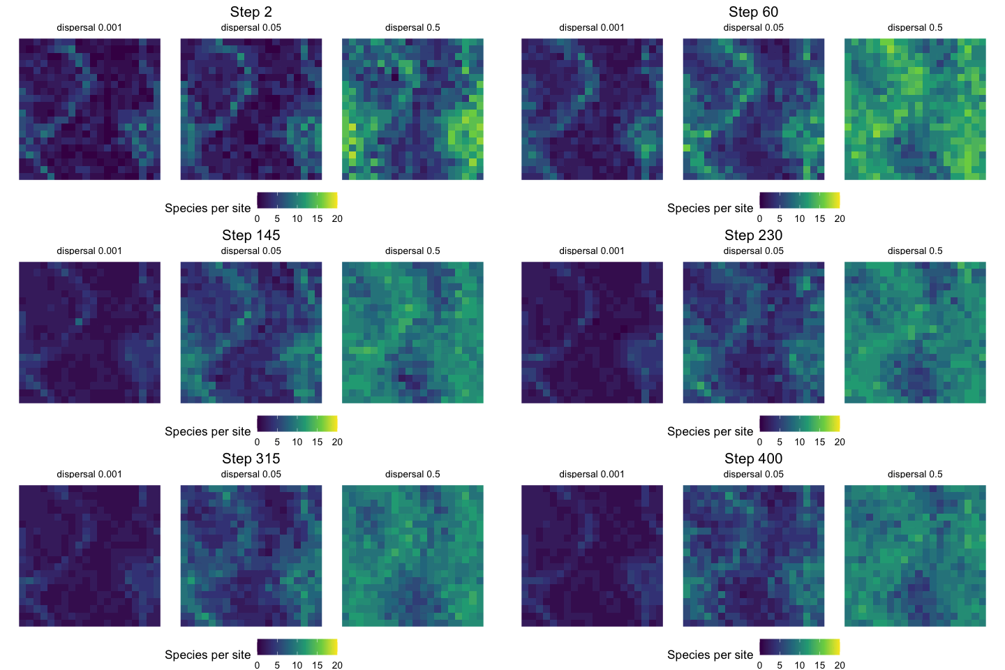
With little dispersal, most sites end with few species. As dispersal increases, immigrants keep species in sites where they could not persist alone, and local richness rises.

Tracking a moving environment

Here the environment stays fixed until step 200, and then the whole map moves one cell every 5 steps, passed to the simulation through env_time. The first panel shows the environment. The others show the mean optimum of the individuals in each site, so a panel that resembles the first one has species matched to their sites. Empty sites are grey.

env_map <- matrix(land$env, 20)
shift <- function(k) c(env_map[, (1:20 + k - 1) %% 20 + 1])
env_time <- sapply(1:400, function(t) shift(max(0, t - 200) %/% 5))
sim <- simulate_metacommunity(land, traits, alpha, dispersal = 0.05, n_steps = 400,
                              env_time = env_time, record_steps = frames)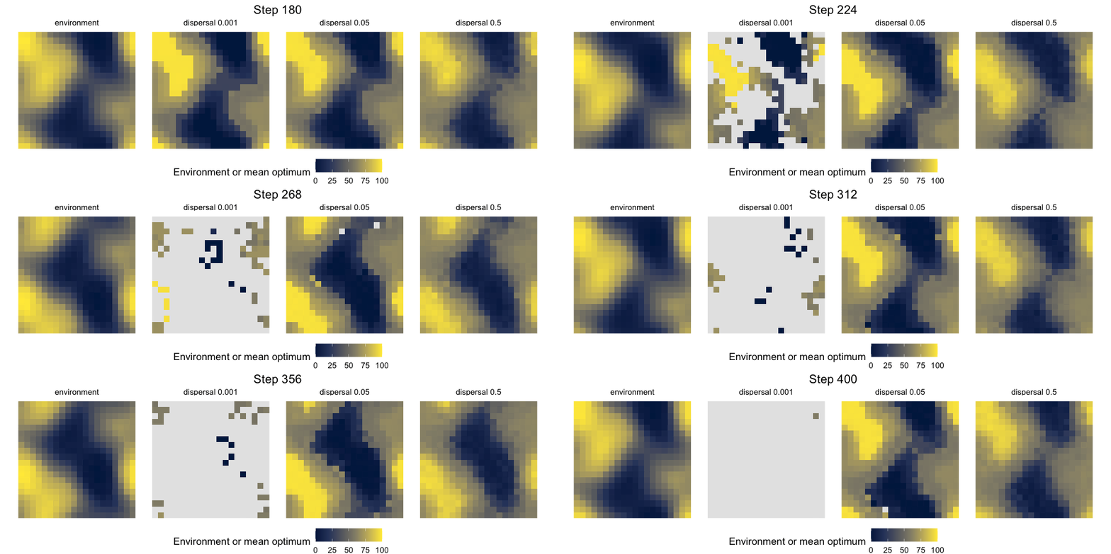

Maps of the environment and of the mean optimum of local communities from step 180 to 400. With dispersal of 0.001 the sites empty after the environment starts to move; with higher dispersal, communities follow the environment.

In this run, at a dispersal rate of 0.001 species cannot keep up: sites become unsuitable faster than they are colonised, and no site is occupied by step 400. At 0.05 and 0.5 communities follow the environment, and the higher rate gives a smoother map, because immigrants blur the differences among neighbouring sites.

Species here have no evolution and no input from outside the landscape, so a species lost from the region does not return.