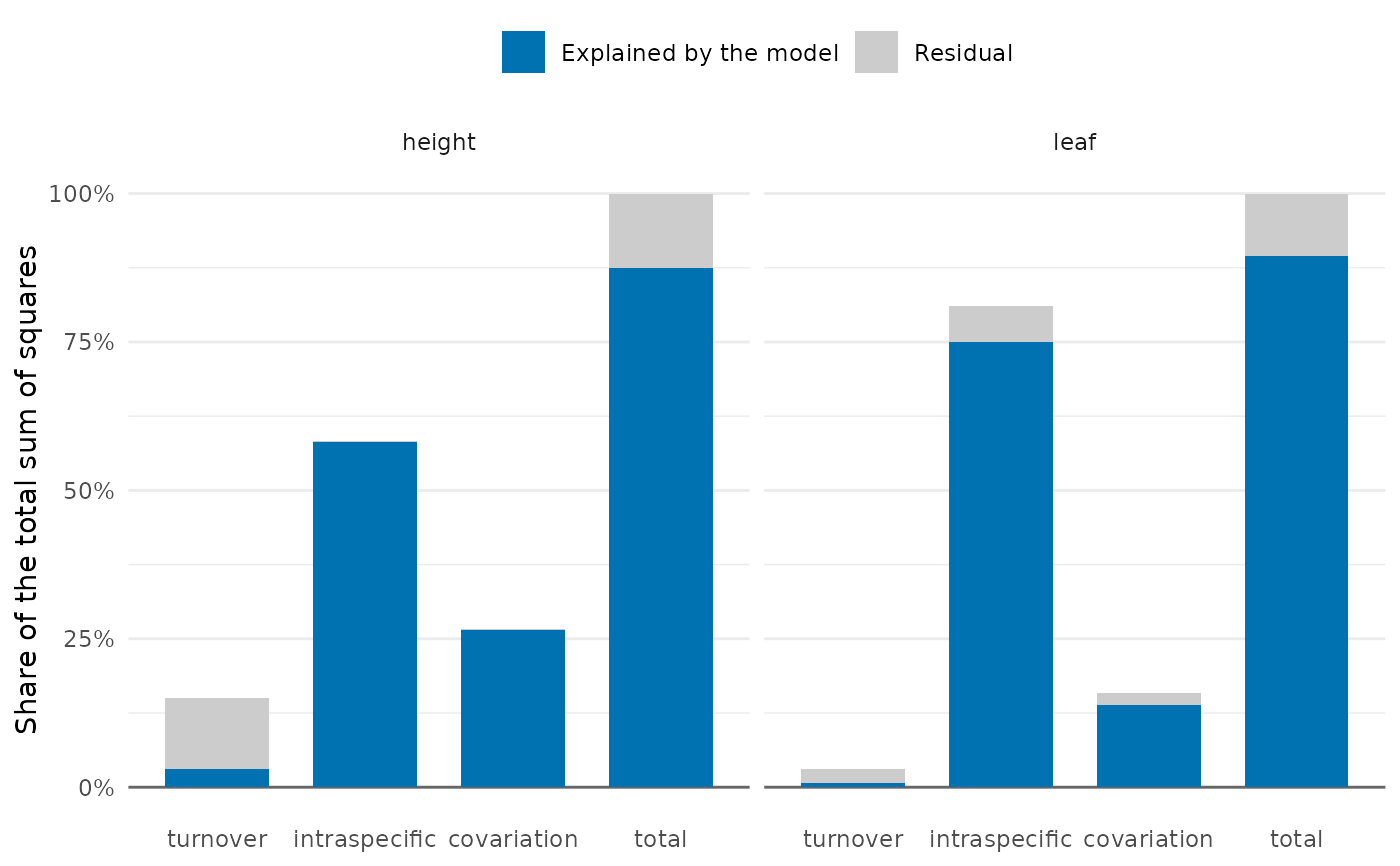
Draws, for each trait, the sums of squares among sites of the community mean due to species
turnover, intraspecific variability, their covariation and the total, from trait_flex().
With an environmental model each bar is split into the part explained by the model and the
residual part. A negative covariation (turnover and intraspecific variability moving the
community mean in opposite directions) is drawn below zero. Needs the package ggplot2.
Arguments
- x
Result of
trait_flex().- relative
If
TRUE(the default), sums of squares are divided by the total sum of squares of each trait, so that traits on different scales can be compared.- colours
Two colours, for the explained and the residual parts (only the first is used without a model). The default is the blue of the Okabe-Ito palette and a light grey, as in
plot.nested_variance().- ...
Not used.
See also
Other trait variation among individuals:
community_index(),
drift_test(),
neighbour_metrics,
nested_variance(),
null_intervals(),
plot.mc_trait_gradient(),
plot.nested_variance(),
plot.trait_rarefaction(),
plot.tstats(),
plot_population_traits(),
population_shifts(),
sample_individuals(),
subsample_individuals(),
trait_densities(),
trait_flex(),
trait_gradient(),
trait_gradient_bayes(),
trait_gradient_phylo(),
trait_gradient_test(),
trait_gradient_weights(),
trait_rarefaction(),
tstats(),
tstats_summary()
Examples
set.seed(1)
ind <- data.frame(site = rep(paste0("s", 1:8), each = 20),
                  species = sample(c("a", "b", "c"), 160, replace = TRUE))
env <- data.frame(site = paste0("s", 1:8), moisture = 1:8)
shift <- env$moisture[match(ind$site, env$site)]
ind$height <- c(a = 10, b = 20, c = 30)[ind$species] + shift + rnorm(160)
ind$leaf <- c(a = 3, b = 2, c = 1)[ind$species] - 0.3 * shift + rnorm(160)
plot(trait_flex(ind, traits = c("height", "leaf"), formula = ~ moisture, env = env))