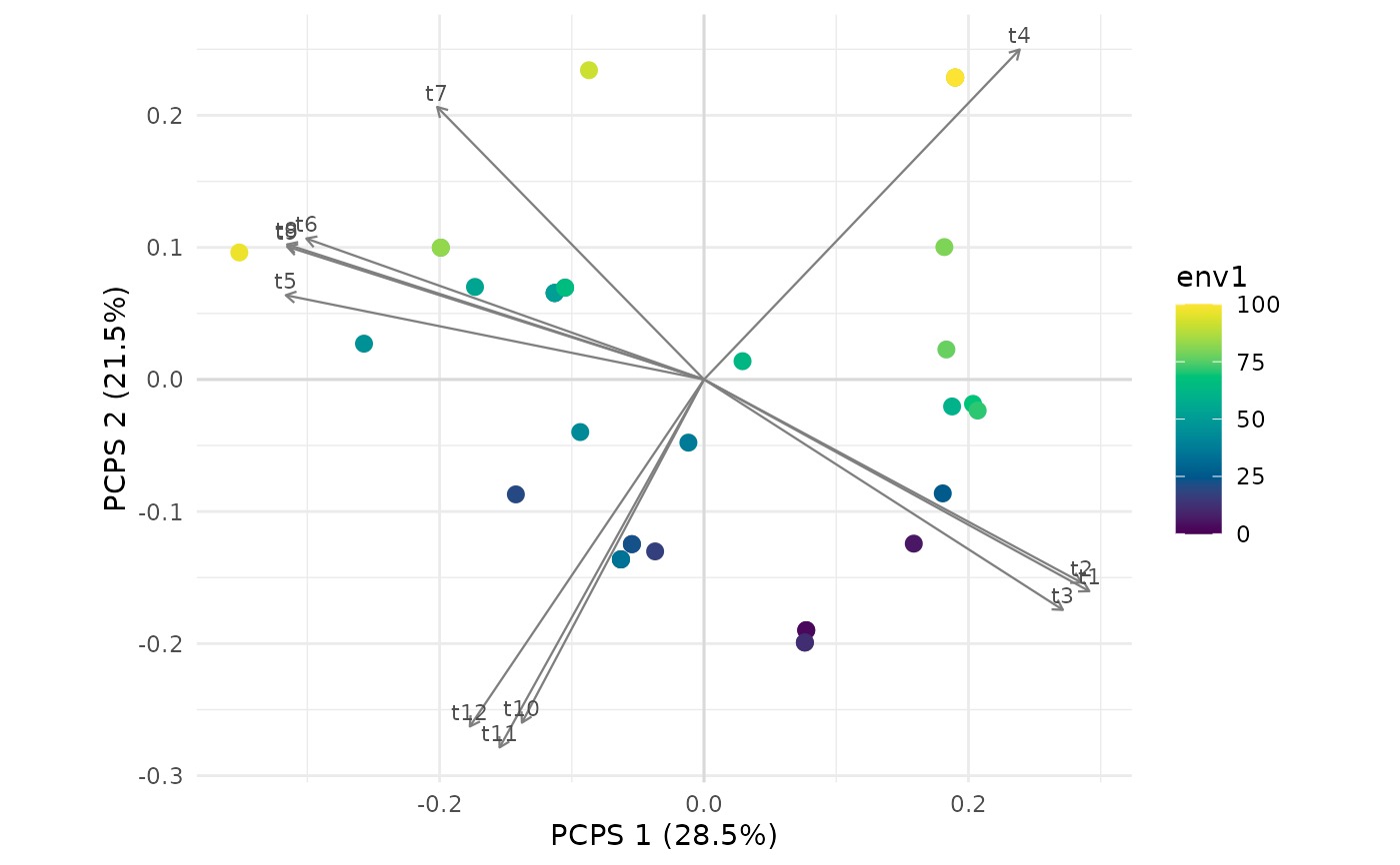
Draws the sites on two principal coordinates of pcps_test(), coloured by a predictor, with
the species as arrows from the correlation of their column of the matrix P with the axes,
as in the biplot of the package PCPS (Debastiani & Duarte 2014). With clades, the species
are drawn as stars coloured by clade, each clade with its outline and name, as in Fig. 1 of
Debastiani & Duarte (2014), which shows which lineages go with which sites.
Arguments
- x
Result of
pcps_test().- axes
The two principal coordinates to draw.
- env
Predictor that colours the sites: a column number or name of the predictors given to
pcps_test(), orNULLfor no colour.- species
Draw the species as arrows.
- species_labels
Write the names of the species at the arrows or stars.
- clades
Optional grouping of the species into clades: a single number k, which cuts the tree into its k deepest clades by splitting, one at a time, the clade whose crown is nearest the root; or a vector of clade names named by species, such as families, in which species left out are drawn in grey without a clade. Each clade with at least three species gets its convex hull.
- palette
Name of a palette of
grDevices::hcl.colors()for the predictor.- point_size
Size of the site points.
- ...
Not used.
References
Debastiani, V. J., & Duarte, L. D. S. (2014). PCPS – an R-package for exploring phylogenetic eigenvectors across metacommunities. Frontiers of Biogeography, 6. doi:10.21425/F5FBG22943
See also
Other the whole tree:
pcc_test(),
pcps_test(),
phylo_beta(),
phylo_beta_test(),
phylo_eigenvectors(),
plot_phylo_beta()
Examples
set.seed(1)
tree <- treeshapesim::sim_tree_shape(12)
traits <- species_traits(tree, lambda = 1, optima_range = c(0, 100), rmax_range = c(0, 30))
env <- seq(0, 100, length.out = 36)
comm <- simulate_static(traits, env, incidence = TRUE)$abundance
plot(pcps_test(comm, tree, env, n_perm = 19))