
Manual review is the most expensive step of the workflow, so the number of clips to validate per site x species is a design decision. sheepdog offers two complementary views of it:
-
Stage 2,
calibration_effort(). The cross-validated AUC of a calibration model as a function of the number of reviewed clips per site x species cell. It answers whether, pooled over all cells, more clips would still improve the calibration. -
Stage 1,
precision_by_bin()andsuggest_thresholds(). Precision by confidence bin and the lowest threshold that reaches a target precision, for each site x species, with flags for bins and thresholds resting on few clips. They show which cells lack support.
This vignette runs both on the simulated example shipped with the package.
Example data
The example holds BirdNET predictions simulated for frog species at
several sites over six months (data-raw/make_example_data.R
in the source repository). False-positive confidences overlap those of
true detections, and false-positive rates differ among species and
sites. The reviewed clips were drawn with the "top" design
(the two highest confidences per site x species x night x hour, up to 80
clips per site x species) and their verdicts come from the simulated
truth. Species with few detections at a site yield fewer than 80 clips
there.
library(sheepdog)
library(dplyr, warn.conflicts = FALSE)

ex <- system.file("extdata", "example", package = "sheepdog")
val_files <- list.files(file.path(ex, "validation"), full.names = TRUE)
basename(val_files)
#> [1] "validation_by_clip_ARA.csv" "validation_by_clip_BAI.csv"
#> [3] "validation_by_clip_NHE.csv" "validation_by_clip_XAR.csv"
read_validations() stacks the tables and keeps the clips
with a verdict and a confidence score, in the form used by the
calibration models:
val <- read_validations(val_files)
#> 2467 reviewed clips (1577 TP / 890 FP) of 8 species at 4 sites.
val |>
  summarise(precision = round(mean(tp), 2), .by = c(site, species)) |>
  tidyr::pivot_wider(names_from = species, values_from = precision)
#> # A tibble: 4 × 9
#>   site  boa_ran den_nan ela_bic lep_fus lep_pod phy_cuv pse_pla sci_nas
#>   <fct>   <dbl>   <dbl>   <dbl>   <dbl>   <dbl>   <dbl>   <dbl>   <dbl>
#> 1 ARA      0.98    0.82    0.91    0       0.91    0.98    0.61    0.81
#> 2 BAI      0.78    0.35    0.94    0       0.79    0.96    0.21    0.42
#> 3 NHE      0.44    0.51    0.8     0.62    0.76    0.89    0.3     0.24
#> 4 XAR      0.71    0.3     0.92    0.6     0.94    0.78    0.12    0.51
The table gives the share of true positives among the reviewed clips of each cell (8 species x 4 sites = 32 cells of 33 to 80 clips). It already shows that the same design yields very different precision across species and sites.
Stage 2: the effort curve
How the curve is built
For each training size n in n_train,
calibration_effort() draws n clips from every site
x species cell (keeping at least five per cell for testing), fits the
model to the drawn clips and computes the AUC on all the remaining
clips. This is repeated n_reps times per n;
repetitions whose fit fails, or with fewer than 50 test clips, are
dropped. The result gives, for each n, the mean and standard
deviation of the AUC across repetitions.
The candidate formulas come from calibration_models(),
and compare_calibration_models() ranks them by 5-fold
cross-validation on all the clips (formulas with random effects need the
‘lme4’ package):
models <- calibration_models()
cv <- compare_calibration_models(val, models)
#> Cross-validation (5 folds) of 5 models...
select(cv, model, auc_mean, auc_sd)
#> # A tibble: 5 × 3
#>   model                auc_mean  auc_sd
#>   <chr>                   <dbl>   <dbl>
#> 1 m4_species_x_site       0.942 0.00564
#> 2 m3_plus_site            0.928 0.00640
#> 3 m2_species_slope        0.916 0.00556
#> 4 m1_species_intercept    0.902 0.00544
#> 5 m0_global               0.862 0.0120
The effort curve below is drawn for the global model
(m0_global, a single logistic regression on the logit of
the score) and for the hierarchical m4_species_x_site
(random slopes by species and a site x species intercept), the structure
used by FrogNet.
The vignette uses few repetitions so that it renders quickly. In real
use keep the default of 50 repetitions (or more): the standard deviation
is itself estimated from n_reps values and is unstable with
few repetitions. Training sizes must stay below the size of the smallest
cell minus five, since at most n - 5 clips of a cell are
used for training whatever the value of n_train.
calibration_effort() warns when a requested size exceeds
that limit, and reports the training size actually used
(n_train_mean), the size of the test set
(n_test_mean) and the repetitions dropped
(n_failed) next to the AUC.
cell_min <- min(count(val, site, species)$n)
cell_min
#> [1] 33
n_train <- c(5, 10, 15, 20, 25)
n_reps  <- 15
The smallest cell holds 33 clips, so the largest training size that
every cell can supply is 28, and n_train stops below it.
Larger sizes would trigger the warning, and n_train_mean
would fall below n_per_cell: the small cells would
contribute fewer clips than requested, and the curve would no longer
describe a uniform effort per cell. To explore larger efforts, draw the
curve on the subset of cells large enough to supply them, keeping in
mind that this subset excludes the species with few detections, often
the hardest to calibrate.
The two curves
eff_m0 <- calibration_effort(val, models$m0_global,
                             n_train = n_train, n_reps = n_reps)
#> Effort curve (15 repetitions per n)...
eff_m0
#> # A tibble: 5 × 6
#>   n_per_cell auc_mean  auc_sd n_train_mean n_test_mean n_failed
#>        <dbl>    <dbl>   <dbl>        <dbl>       <dbl>    <int>
#> 1          5    0.862 0.00188            5        2307        0
#> 2         10    0.860 0.00217           10        2147        0
#> 3         15    0.862 0.00348           15        1987        0
#> 4         20    0.860 0.00414           20        1827        0
#> 5         25    0.860 0.00611           25        1667        0
eff_m4 <- calibration_effort(val, models$m4_species_x_site,
                             n_train = n_train, n_reps = n_reps)
#> Effort curve (15 repetitions per n)...
eff_m4
#> # A tibble: 5 × 6
#>   n_per_cell auc_mean  auc_sd n_train_mean n_test_mean n_failed
#>        <dbl>    <dbl>   <dbl>        <dbl>       <dbl>    <int>
#> 1          5    0.918 0.00896            5        2307        0
#> 2         10    0.930 0.00449           10        2147        0
#> 3         15    0.934 0.00325           15        1987        0
#> 4         20    0.936 0.00331           20        1827        0
#> 5         25    0.937 0.00335           25        1667        0
The draws depend only on seed, n_train,
n_reps and the data, not on the formula, so with the same
arguments both curves are computed on the same training and test sets
and can be compared repetition by repetition.
effort <- bind_rows(m0_global = eff_m0,
                    m4_species_x_site = if (has_lme4) eff_m4,
                    .id = "model")

library(ggplot2)
ggplot(effort, aes(n_per_cell, auc_mean, colour = model)) +
  geom_line() +
  geom_pointrange(aes(ymin = auc_mean - auc_sd, ymax = auc_mean + auc_sd),
                  position = position_dodge(width = 2)) +
  labs(x = "Reviewed clips per site x species (training)",
       y = "Cross-validated AUC (mean ± sd)", colour = "Model") +
  theme_minimal(base_size = 11) +
  theme(legend.position = "bottom")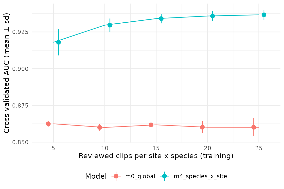
Reading the curve
Which formula. The curve belongs to a model, not to
the data. The mean AUC of the global model stays between 0.86 and 0.862
at every training size: it has only two parameters, which are estimated
well from a few clips per cell, and more clips cannot correct its
structural limitation, that one score-to-probability curve is shared by
all species and sites. The hierarchical model is higher at every size
(0.918 with 5 clips per cell, 0.936 with 20 and 0.937 with 25) and,
unlike the global model, it gains from additional clips, because each
clip also informs the species- and site-specific terms. The gap between
the curves is the gain from modelling how species and sites differ; its
size, not only the height of either curve, is what the choice of formula
rests on. Draw the curve for the formula that
compare_calibration_models() selects (or that
calibrate() refits), with m0_global as a
baseline.
Where it flattens. Beyond the training size at which the mean AUC stops increasing, extra clips in every cell add little discrimination. With a tolerance of 0.005 below the best mean AUC of each curve (an illustrative choice, not a rule of the package), the global model is flat from 5 clips per cell and the hierarchical model from 15. For the hierarchical model the gain per clip falls with effort: the first 5 extra clips per cell (from 5 to 10) add 0.012 to the mean AUC, and the next 15 (from 10 to 25) add 0.007 in total. The first clips of a cell fix its intercept and slope; the later ones only refine them. Whether the curve keeps rising beyond 28 clips per cell cannot be assessed with every cell in the curve (see above). Small dips in the mean between neighbouring training sizes are within the spread of the repetitions and should not be read as losses.
The variability across repetitions. At small
n the standard deviation measures how much the calibration
depends on which clips were reviewed; a large spread means that
a single validation round of that size may produce a poor model by
chance. For the hierarchical model it is largest with 5 clips per cell
(sd = 0.009) and halves by 15. The spread can also grow with n
for a different reason: the test set is what is left of each cell, so it
shrinks as n grows (n_test_mean; with 25 training
clips per cell, 1667 of the 2467 clips remain for testing). The standard
deviation of the global model, which gains nothing from extra clips,
rises from 0.002 to 0.006 for that reason alone.
AUC measures discrimination (whether true detections score higher
than false ones), not whether the calibrated probabilities are accurate.
A curve that has flattened does not imply that the species- or
site-specific curves of plot_calibration() are well
estimated in every cell; that is what the per-cell view of stage 1
checks.
Stage 1: which cells lack support
The effort curve pools all cells. precision_by_bin() and
suggest_thresholds() work cell by cell on the
validation_by_clip.csv tables (the output of
post_validation()), so they read the raw tables rather than
the output of read_validations():
val_raw <- purrr::map(val_files, readr::read_csv, show_col_types = FALSE) |>
  purrr::list_rbind()

prec <- precision_by_bin(val_raw, min_n = 15)
prec |>
  filter(site == "BAI", species_folder %in% c("phy_cuv", "pse_pla")) |>
  mutate(precision = round(precision, 2)) |>
  select(species_folder, bin, n = n_reviewed, precision) |>
  tidyr::pivot_wider(names_from = species_folder,
                     values_from = c(n, precision)) |>
  arrange(bin)
#> # A tibble: 9 × 5
#>   bin       n_phy_cuv n_pse_pla precision_phy_cuv precision_pse_pla
#>   <fct>         <int>     <int>             <dbl>             <dbl>
#> 1 [0.1,0.2)         1        NA               0               NA
#> 2 [0.2,0.3)         1         5               0                0.4
#> 3 [0.3,0.4)        NA         6              NA                0
#> 4 [0.4,0.5)         2        10               0.5              0.3
#> 5 [0.5,0.6)         4        18               1                0.22
#> 6 [0.6,0.7)         5        11               1                0.45
#> 7 [0.7,0.8)        12        19               1                0.11
#> 8 [0.8,0.9)        31         8               1                0
#> 9 [0.9,1]          24         3               1                0.33
A bin is flagged low_support when it holds fewer than
min_n reviewed clips (here, bins with n below
15). The two cells shown differ in how the flags should be read. For
phy_cuv at BAI the reviewed clips concentrate in the upper
bins, as expected from the "top" design, and precision
there is high; the flagged low bins matter only if the study needs a low
threshold. For pse_pla at BAI the clips spread over the whole
range and precision stays low at high scores, including the upper bins
that reach min_n: the classifier confuses this species at
high scores, and more clips would not change that.
suggest_thresholds() returns, for each cell, the lowest
confidence at which precision reaches target_precision with
at least min_n clips above it (NA when no cut
does):
thr <- suggest_thresholds(val_raw, target_precision = 0.90, min_n = 15)
thr |>
  mutate(threshold = if_else(is.na(threshold), "-",
                             format(threshold, nsmall = 2))) |>
  select(site, species_folder, threshold) |>
  tidyr::pivot_wider(names_from = species_folder, values_from = threshold)
#> # A tibble: 4 × 9
#>   site  boa_ran den_nan ela_bic lep_fus lep_pod phy_cuv pse_pla sci_nas
#>   <chr> <chr>   <chr>   <chr>   <chr>   <chr>   <chr>   <chr>   <chr>
#> 1 ARA   0.36    0.56    0.13    -       0.10    0.19    -       0.69
#> 2 BAI   0.39    -       0.23    -       0.32    0.11    -       -
#> 3 NHE   0.55    0.77    0.26    -       0.35    0.22    -       -
#> 4 XAR   0.58    -       0.11    0.70    0.16    0.27    -       -
The target is reached in 20 of the 32 cells. A missing threshold has two possible causes, and they call for opposite decisions: too few reviewed clips at high scores (more review may help) or low precision even at high scores (more review will not). To tell them apart, count the high-score clips reviewed in each cell, their precision, and how many high-score detections in the complete selection tables were not reviewed:
conf_high <- 0.7   # example: what counts as a high score
min_n     <- 15

detections <- suppressMessages(
  read_selection_tables(file.path(ex, "birdnet"))) |>
  mutate(species = gsub("-", "_", sub("^.*_", "", species_code)))

support <- val |>
  mutate(across(c(site, species), as.character)) |>
  summarise(n_fp      = sum(tp == 0),
            n_high    = sum(confidence >= conf_high),
            prec_high = round(mean(tp[confidence >= conf_high]), 2),
            .by = c(site, species)) |>
  left_join(detections |>
              summarise(n_high_all = sum(confidence >= conf_high),
                        .by = c(site, species)),
            by = c("site", "species")) |>
  left_join(select(thr, site, species = species_folder, threshold),
            by = c("site", "species")) |>
  mutate(unreviewed_high = n_high_all - n_high,
         diagnosis = case_when(
           !is.na(threshold)        ~ "reached",
           unreviewed_high < min_n  ~ "exhausted",
           prec_high < 0.5          ~ "unreliable",
           .default = "review more"
         )) |>
  select(site, species, n_fp, n_high, prec_high, unreviewed_high,
         diagnosis) |>
  arrange(diagnosis, species, site)
print(support, n = Inf)
#> # A tibble: 32 × 7
#>    site  species  n_fp n_high prec_high unreviewed_high diagnosis
#>    <chr> <chr>   <int>  <int>     <dbl>           <int> <chr>
#>  1 ARA   lep_fus    33      1      0                  0 exhausted
#>  2 BAI   lep_fus    56      3      0                  0 exhausted
#>  3 ARA   boa_ran     2     59      1                122 reached
#>  4 BAI   boa_ran    18     45      1                 25 reached
#>  5 NHE   boa_ran    45     26      0.96              18 reached
#>  6 XAR   boa_ran    23     49      0.98              29 reached
#>  7 ARA   den_nan    14     35      0.94              57 reached
#>  8 NHE   den_nan    39     33      0.82              47 reached
#>  9 ARA   ela_bic     7     61      1                 42 reached
#> 10 BAI   ela_bic     5     55      1                 51 reached
#> 11 NHE   ela_bic    16     53      1                 65 reached
#> 12 XAR   ela_bic     6     57      1                 46 reached
#> 13 XAR   lep_fus    32     16      0.94              17 reached
#> 14 ARA   lep_pod     7     62      1                 48 reached
#> 15 BAI   lep_pod    12     39      1                 12 reached
#> 16 NHE   lep_pod    19     53      1                 53 reached
#> 17 XAR   lep_pod     5     64      1                 91 reached
#> 18 ARA   phy_cuv     2     71      1                 64 reached
#> 19 BAI   phy_cuv     3     67      1                 68 reached
#> 20 NHE   phy_cuv     9     63      1                111 reached
#> 21 XAR   phy_cuv    18     59      0.98              39 reached
#> 22 ARA   sci_nas    15     40      0.92              34 reached
#> 23 BAI   den_nan    52     23      0.7               21 review more
#> 24 XAR   den_nan    56     27      0.63              20 review more
#> 25 NHE   lep_fus    30     18      0.78              19 review more
#> 26 ARA   pse_pla    31     26      0.62              23 review more
#> 27 BAI   sci_nas    46     30      0.7               30 review more
#> 28 NHE   sci_nas    61     21      0.52              42 review more
#> 29 XAR   sci_nas    39     36      0.69              39 review more
#> 30 BAI   pse_pla    63     30      0.1               16 unreliable
#> 31 NHE   pse_pla    56     37      0.32              61 unreliable
#> 32 XAR   pse_pla    70     26      0.15              34 unreliable
A cell is "reached" when
suggest_thresholds() found a threshold. The other labels
use illustrative cut-offs (conf_high, min_n
and a precision of 0.5 at high scores); set them from the precision the
study needs. In this example they separate three groups of cells that
lack support:
-
"review more": den_nan at BAI, den_nan at XAR, lep_fus at NHE, pse_pla at ARA, sci_nas at BAI, sci_nas at NHE, sci_nas at XAR. Precision at high scores is intermediate and unreviewed high-score detections remain, so a further round of review restricted to high scores in these cells may reveal a cut that reaches the target. -
"exhausted": lep_fus at ARA, lep_fus at BAI. The"top"design has already taken almost every high-score detection of these cells; more effort cannot add support. Treat the species at that site as poorly calibrated. In this example these cells have 0 true positives among their reviewed clips in total (seen_fpbelow). -
"unreliable": pse_pla at BAI, pse_pla at NHE, pse_pla at XAR. Most high-score detections are false positives; more review would only confirm it. These cells call for retraining the classifier (with the clips ofretraining_clips()) rather than for more validation.
The column n_fp deserves a look of its own. The
calibration slope is estimated from the contrast between true and false
positives, so a cell with few false positives (here as few as 2) carries
little information about the low end of its calibration curve, even when
its total number of reviewed clips is large. At the other extreme, a
cell whose reviewed clips are all false positives (lep_fus at ARA,
lep_fus at BAI) gives no information on true detections at all; it may
be a site where the species is absent. These are interpretations of the
model structure, not flags computed by the package.
The practical decision
Read the two views together:
- If the effort curve of the chosen model is still rising at the current number of clips per cell, review more clips in every cell: the pooled calibration is limited by the overall effort.
- If the curve has flattened but some cells lack support in stage 1, review more clips only in those cells, and target the confidence range where support is missing. Clips in cells that are already well supported add little.
- If a cell is
"exhausted"(no high-score detections left to review) or"unreliable"(low precision even at high scores), more validation cannot help. Treat the species at that site as poorly calibrated, as FrogNet did with the six species left out of the community matrices (seevignette("frognet-workflow")).
Two caveats apply. First, the curve depends on the formula: a
hierarchical formula needs ‘lme4’, and its curve can differ markedly
from that of the global model, so draw it for the model that will be
used. Second, the curve depends on how the clips were chosen. The
training and test clips of calibration_effort() are drawn
from the same reviewed pool, so the AUC describes discrimination among
clips selected by the same design. With the "top" design
the pool over-represents high scores; the AUC is conditional on that
design and is not an estimate of the false-positive rate of all
detections. For that, use the "random_detections" design,
which follows the observation-confirmation design of Chambert et al. (2015) (see
vignette("crywolf-integration")).
The effort curve can also be drawn inside the whole calibration
stage, with calibrate(..., effort_curve = TRUE); it is then
computed for the best model of the cross-validation and written to
effort_curve.csv. The arguments effort_n and
effort_reps set the training sizes and the number of
repetitions.
sites <- c("ARA", "BAI", "NHE", "XAR")
res <- calibrate(
  validation_files  = val_files,
  prediction_tables = setNames(
    file.path(ex, "birdnet", sites, "BirdNET_SelectionTable.txt"), sites),
  output_dir   = file.path(tempdir(), "calibration"),
  effort_curve = TRUE, effort_n = c(5, 10, 15, 20, 25),
  effort_reps  = 50
)
res$effort