Choosing a sampling design

select_clips() offers three sampling designs, set by sampling_mode. They answer different questions, and a validation sample drawn for one purpose is generally not valid for another. This vignette states what each design is for, runs the three on the example data shipped with the package and compares the clips they select.

`sampling_mode`	unit drawn	selection	use
`"top"`	prediction	highest confidence per stratum	classifier retraining; score-to-probability calibration
`"random_detections"`	occasion with a detection	random, within score-independent strata	false-positive rates, observation-confirmation design
`"random_recordings"`	recording or minute	random, among all recorded	false-positive and false-negative rates, multiple-method design

Example data

The example consists of simulated BirdNET selection tables (Raven format) of anuran calls at several sites over six months (October 2021 to March 2022), plus the list of every recording made (recordings.csv), including those without any prediction. The audio files do not exist: Begin Path points to a fictitious network drive. Because select_clips() never reads audio, this does not prevent any of the steps below.

library(sheepdog)
suppressPackageStartupMessages(library(dplyr))

ex   <- system.file("extdata", "example", package = "sheepdog")
pred <- suppressMessages(read_selection_tables(file.path(ex, "birdnet")))
recs <- readr::read_csv(file.path(ex, "recordings.csv"),
                        show_col_types = FALSE)
count(pred, site)
#> # A tibble: 4 × 2
#>   site      n
#>   <chr> <int>
#> 1 ARA    1753
#> 2 BAI    1427
#> 3 NHE    2507
#> 4 XAR    1866

There are 7553 predictions of 8 species at 4 sites, from 354 recordings of 300 s. Recording effort differs among sites:

count(recs, site, name = "recordings")
#> # A tibble: 4 × 2
#>   site  recordings
#>   <chr>      <int>
#> 1 ARA           90
#> 2 BAI           90
#> 3 NHE           90
#> 4 XAR           84

Throughout, the occupancy analysis is assumed to treat a prediction with confidence $\geq$ 0.5 as a detection:

threshold <- 0.5
above <- filter(pred, confidence >= threshold)
nrow(above)
#> [1] 4738

`"top"`: the highest scores

"top" keeps the n_top predictions with the highest confidence in each site × species × night × hour stratum. Predictions below min_confidence are discarded first.

top <- select_clips(pred, sampling_mode = "top", n_top = 1,
                    min_confidence = threshold)
#> Sampling mode: top (occasion = file).
#> 2815 predictions dropped by the filter confidence < 0.5.
#> 1876 clips selected (top 1 per site x species x night x hour) of 8 species.

This design is appropriate for two purposes. First, retraining the classifier, where confirmed high-score examples of each species are the most useful additions to the training set. Second, the score-to-probability calibration of calibrate(): the calibration model describes the probability that a prediction is correct conditional on its score, so selecting clips by score does not bias it, provided the selected clips span the range of scores of interest.

"top" is not a probability sample, and inclusion_prob is NA. It must not be used to estimate false-positive rates for occupancy models. Clips with the highest scores contain fewer false positives than a random sample of detections, so the proportion of negatives among them underestimates the false-positive rate of the detections that enter the detection history.

`"random_detections"`: observation-confirmation design

In the observation-confirmation design (Chambert et al. 2015), a random subset of the occasions with a detection is checked, and every detection of a checked occasion is confirmed or rejected. "random_detections" implements it as follows:

A candidate occasion is an occasion with at least one prediction of the species with confidence $\geq$ threshold. The occasion is the sampling unit of the occupancy model, set by occasion_unit: the whole recording ("file") or one minute of it ("minute").
n_top candidate occasions are drawn at random in each site × species × night × hour stratum. The strata do not depend on the score, so every detection has a known, non-zero probability of being checked.
Every prediction $\geq$ threshold of a drawn occasion becomes a clip.

threshold is required and must equal the threshold of the occupancy analysis; otherwise the occasions drawn are not the occasions scored as detections in the model.

With occasion_unit = "file":

rd_file <- select_clips(pred, sampling_mode = "random_detections",
                        occasion_unit = "file", threshold = threshold,
                        n_top = 1)
#> Sampling mode: random_detections (occasion = file).
#> 1876 occasions drawn (1 per site x species_code x night x recording_hour) among 1876 with a prediction >= 0.5.
#> 4738 clips (every prediction >= 0.5 of the 1876 occasions drawn).
table(rd_file$inclusion_prob)
#> 
#>    1 
#> 4738

files_per_stratum <- recs |>
  mutate(stamp = sub(".*_(\\d{8})_(\\d{2}).*", "\\1_\\2", source_audio)) |>
  count(site, stamp)
max(files_per_stratum$n)
#> [1] 1

In the example data each site × night × hour holds at most 1 recording, so each stratum contains at most one candidate file and the first-stage draw keeps all of them (inclusion_prob = 1). The same applies to any recording schedule with one file per hour. Subsampling then requires a coarser stratum, minute occasions or the limits described under Limiting the effort.

The strata argument sets the stratum of the draw: "night_hour" (the default), "night" or "site_species". With strata = "night", the files of a night compete with each other, and one is drawn per site × species × night:

rd_night <- select_clips(pred, sampling_mode = "random_detections",
                         occasion_unit = "file", threshold = threshold,
                         n_top = 1, strata = "night")
#> Sampling mode: random_detections (occasion = file).
#> 1343 occasions drawn (1 per site x species_code x night) among 1876 with a prediction >= 0.5.
#> 3339 clips (every prediction >= 0.5 of the 1343 occasions drawn).
summary(rd_night$inclusion_prob)
#>    Min. 1st Qu.  Median    Mean 3rd Qu.    Max. 
#>  0.5000  0.5000  1.0000  0.7929  1.0000  1.0000

Besides "night_hour", "night" and "site_species", the presets "hour" (pooling the nights), "week" and "month" spread the draw over the diel cycle or the season. With strata = "month", the files of a month compete with each other:

rd_month <- select_clips(pred, sampling_mode = "random_detections",
                         occasion_unit = "file", threshold = threshold,
                         n_top = 2, strata = "month")
#> Sampling mode: random_detections (occasion = file).
#> 332 occasions drawn (2 per site x species_code x month) among 1876 with a prediction >= 0.5.
#> 780 clips (every prediction >= 0.5 of the 332 occasions drawn).
summary(rd_month$inclusion_prob)
#>    Min. 1st Qu.  Median    Mean 3rd Qu.    Max. 
#>  0.1333  0.1429  0.1429  0.2028  0.1667  1.0000

strata also takes a vector of column names, for strata defined by the user. Any column added to the predictions before the call can be used. Since site and species are always part of the strata, a useful column varies within a site: the rain of the night, a recorder when a site has several, or, as here, the moon phase, approximated from the date of the night (days since a reference new moon, modulo the synodic month of 29.53 days) and crossed with the month.

moon_phase <- function(night) {
  days <- as.numeric(as.Date(night, "%Y%m%d") - as.Date("2000-01-06"))
  cut(days %% 29.530588, breaks = c(0, 7.38, 14.77, 22.15, 29.54),
      labels = c("new", "first_quarter", "full", "last_quarter"),
      include.lowest = TRUE)
}
# the date (YYYYMMDD) comes from the name of the recording
rd_moon <- pred |>
  mutate(date = regmatches(begin_path, regexpr("\\d{8}(?=_\\d{6})",
                                                begin_path, perl = TRUE)),
         moon = as.character(moon_phase(date))) |>
  select_clips(sampling_mode = "random_detections", occasion_unit = "file",
               threshold = threshold, n_top = 1,
               strata = c("month", "moon"))
#> Sampling mode: random_detections (occasion = file).
#> 581 occasions drawn (1 per site x species_code x month x moon) among 1876 with a prediction >= 0.5.
#> 1419 clips (every prediction >= 0.5 of the 581 occasions drawn).
rd_moon |>
  distinct(site, species_code, occasion_id) |>
  nrow()
#> [1] 581

site and species_code are always part of the strata, so that inclusion_prob stays exact when target_total or max_per_species draw again within site × species. The strata must not depend on the score: select_clips() refuses confidence and rank, and every stratum column must be constant within an occasion. Any stratum that meets these conditions is compatible with the observation-confirmation design.

With occasion_unit = "minute", a stratum holds up to five candidate minutes per recording, and one is drawn:

rd <- select_clips(pred, sampling_mode = "random_detections",
                   occasion_unit = "minute", threshold = threshold,
                   n_top = 1)
#> Sampling mode: random_detections (occasion = minute).
#> 1876 occasions drawn (1 per site x species_code x night x recording_hour) among 3824 with a prediction >= 0.5.
#> 2288 clips (every prediction >= 0.5 of the 1876 occasions drawn).

occasion_id identifies the occasion, n_detections_occasion counts the predictions $\geq$ threshold of the species in it, and inclusion_prob is the probability that the occasion was drawn:

rd |>
  select(site, species_code, occasion_id, rank, confidence,
         n_detections_occasion, inclusion_prob) |>
  head(4)
#> # A tibble: 4 × 7
#>   site  species_code          occasion_id  rank confidence n_detections_occasion
#>   <chr> <chr>                 <chr>       <int>      <dbl>                 <int>
#> 1 ARA   Boana raniceps_boa-r… ARA01_2021…     1      0.504                     1
#> 2 ARA   Boana raniceps_boa-r… ARA01_2021…     1      0.586                     1
#> 3 ARA   Boana raniceps_boa-r… ARA01_2021…     1      0.924                     2
#> 4 ARA   Boana raniceps_boa-r… ARA01_2021…     2      0.796                     2
#> # ℹ 1 more variable: inclusion_prob <dbl>
count(rd, inclusion_prob)
#> # A tibble: 5 × 2
#>   inclusion_prob     n
#>            <dbl> <int>
#> 1          0.2      36
#> 2          0.25    176
#> 3          0.333   502
#> 4          0.5     764
#> 5          1       810

inclusion_prob is $\min(n_\mathrm{top}, N) / N$ , where $N$ is the number of candidate occasions in the stratum. Because every detection of a drawn occasion is cut, the number of clips per occasion equals n_detections_occasion:

per_occasion <- count(rd, site, species_code, occasion_id,
                      n_detections_occasion, name = "n_clips")
all(per_occasion$n_clips == per_occasion$n_detections_occasion)
#> [1] TRUE

This check is worth repeating on the validation table before passing it to an occupancy model: a clip missing from an occasion breaks the assumption that all of its detections were confirmed.

`"random_recordings"`: multiple-method design

In the multiple-method design (Miller et al. 2011), a second, unambiguous method (here, annotation by ear of whole recordings) is applied to a random subset of the sampling units, irrespective of whether the classifier detected anything. This provides information on false negatives as well as false positives. "random_recordings" draws recordings (or minutes, with occasion_unit = "minute") among all those recorded, with or without predictions, in proportion to the effort at each site: recording_fraction of the recordings of each site, or a fixed n_recordings_per_site.

The draw needs the list of every recording. By default it is obtained by listing the audio folders that appear in Begin Path, which omits folders without any prediction and fails here because the audio files do not exist. The recordings argument supplies the list instead:

rr <- select_clips(pred, sampling_mode = "random_recordings",
                   recordings = file.path(ex, "recordings.csv"),
                   recording_fraction = 0.1, recording_duration = 300,
                   species = "boa-ran")
#> Sampling mode: random_recordings (occasion = file).
#> 354 recordings listed at 4 site(s).
#> Filter of 1 species: 7553 -> 874 predictions.
#> 35 file(s) drawn among 354 recorded, to annotate 1 species.
rr |>
  select(site, species_code, clip_file, clip_start, clip_end,
         confidence, inclusion_prob) |>
  head(3)
#> # A tibble: 3 × 7
#>   site  species_code     clip_file clip_start clip_end confidence inclusion_prob
#>   <chr> <chr>            <chr>          <dbl>    <dbl>      <dbl>          <dbl>
#> 1 ARA   Boana raniceps_… rec_ARA_…          0      300         NA            0.1
#> 2 ARA   Boana raniceps_… rec_ARA_…          0      300         NA            0.1
#> 3 ARA   Boana raniceps_… rec_ARA_…          0      300         NA            0.1
count(rr, site)
#> # A tibble: 4 × 2
#>   site      n
#>   <chr> <int>
#> 1 ARA       9
#> 2 BAI       9
#> 3 NHE       9
#> 4 XAR       8

The number drawn per site follows its recording effort: with recording_fraction = 0.1, the site with the fewest recordings (XAR, 84) contributes 8 recordings, and inclusion_prob is the fraction drawn at that site. The default recording_fraction = 0.01 suits large projects: with fewer than 150 recordings per site it draws a single recording per site, so small projects should raise it or set n_recordings_per_site.

Each clip is a whole recording (or minute); confidence is NA and rank is NA. recording_duration sets clip_end; without it, clip_end is NA for whole recordings and minute occasions require reading the files with the ‘av’ package. The recording is copied once per species to annotate, so that each copy receives a verdict for one species in that species’ folder. Without species, every species with predictions is included, which multiplies the listening effort by the number of species:

rr_all <- suppressMessages(
  select_clips(pred, sampling_mode = "random_recordings",
               recordings = file.path(ex, "recordings.csv"),
               recording_fraction = 0.1, recording_duration = 300)
)
c(recordings = n_distinct(rr_all$occasion_id), clips = nrow(rr_all))
#> recordings      clips 
#>         35        280

Restrict species to the species that will actually be annotated. Recordings of "random_recordings" are not confirmations of detections and are handled differently downstream (see vignette("crywolf-integration")).

Comparing the selected scores

The practical difference between "top" and "random_detections" is visible in the confidence of the clips they select. The reference is the distribution of all predictions $\geq$ threshold, i.e. the detections that enter the detection history. Clips from "random_detections" are weighted by 1 / inclusion_prob (design weights), because occasions in strata with many candidates have a lower probability of being drawn.

wquantile <- function(x, w = rep(1, length(x)),
                      probs = c(0.1, 0.25, 0.5, 0.75, 0.9)) {
  o  <- order(x)
  cw <- cumsum(w[o]) / sum(w)
  setNames(x[o][vapply(probs, \(p) which(cw >= p)[1], integer(1))],
           paste0(probs * 100, "%"))
}

score_quantiles <- rbind(
  `all >= threshold`  = wquantile(above$confidence),
  random_detections   = wquantile(rd$confidence, 1 / rd$inclusion_prob),
  top                 = wquantile(top$confidence)
)
round(score_quantiles, 3)
#>                     10%   25%   50%   75%   90%
#> all >= threshold  0.547 0.616 0.725 0.836 0.912
#> random_detections 0.545 0.617 0.725 0.831 0.907
#> top               0.592 0.687 0.809 0.897 0.948

The weighted quantiles of "random_detections" track those of all detections (median 0.72 against 0.72), whereas "top" is shifted upwards (median 0.81). To the extent that false positives receive lower scores than true detections, as they do on average in the simulated data (although the two distributions overlap), a false-positive rate estimated from the "top" clips is biased low.

library(ggplot2)

wecdf <- function(x, w, design) {
  o <- order(x)
  tibble(confidence = x[o], ecdf = cumsum(w[o]) / sum(w), design = design)
}
curves <- bind_rows(
  wecdf(above$confidence, rep(1, nrow(above)), "all >= threshold"),
  wecdf(rd$confidence, 1 / rd$inclusion_prob, "random_detections"),
  wecdf(top$confidence, rep(1, nrow(top)), "top")
)

ggplot(curves, aes(confidence, ecdf, colour = design)) +
  geom_step() +
  labs(x = "Confidence", y = "Cumulative proportion", colour = NULL) +
  theme_minimal() +
  theme(legend.position = "bottom")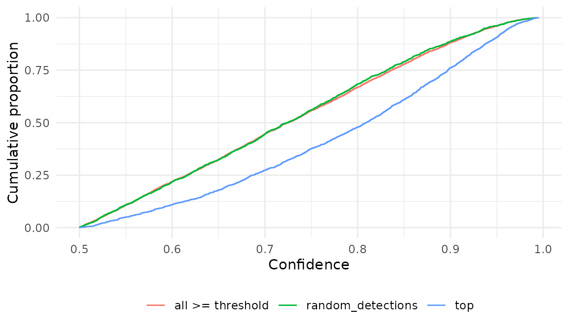

Empirical cumulative distribution of confidence for all detections, random_detections clips and top clips.

Limiting the effort

target_total, max_per_species and balance_by_hour cap the number of units to review after the stratified draw. Their effect differs among designs:

target_total sets the total per site, split evenly among species by water filling (species with fewer units than their share enter whole, and the surplus goes to the others). In "top" it counts clips; in "random_detections" it counts occasions, each of which may yield several clips.
max_per_species sets a fixed limit per site × species. It is ignored when target_total is set.
balance_by_hour = TRUE draws round-robin across the hours of the day within each species, so that the reviewed sample covers the diel cycle.
In "random_recordings" the effort is set by recording_fraction or n_recordings_per_site; target_total and max_per_species are ignored with a warning.

target <- 40
top_cap <- select_clips(pred, sampling_mode = "top", n_top = 1,
                        min_confidence = threshold, target_total = target)
#> Sampling mode: top (occasion = file).
#> 2815 predictions dropped by the filter confidence < 0.5.
#> 1876 clips selected (top 1 per site x species x night x hour) of 8 species.
#> Target of 40 clips per site (balanced by species and hour): 1876 -> 160 clips.
rd_cap  <- select_clips(pred, sampling_mode = "random_detections",
                        occasion_unit = "minute", threshold = threshold,
                        n_top = 1, target_total = target)
#> Sampling mode: random_detections (occasion = minute).
#> 1876 occasions drawn (1 per site x species_code x night x recording_hour) among 3824 with a prediction >= 0.5.
#> Target of 40 occasions per site (balanced by species and hour): 1876 -> 160 occasions.
#> 191 clips (every prediction >= 0.5 of the 160 occasions drawn).

rd_cap |>
  distinct(site, species_code, occasion_id) |>
  count(site, name = "occasions") |>
  left_join(count(rd_cap, site, name = "clips"), by = "site") |>
  left_join(count(top_cap, site, name = "top_clips"), by = "site")
#> # A tibble: 4 × 4
#>   site  occasions clips top_clips
#>   <chr>     <int> <int>     <int>
#> 1 ARA          40    49        40
#> 2 BAI          40    47        40
#> 3 NHE          40    50        40
#> 4 XAR          40    45        40

The same target of 40 units per site yields 160 clips in "top" but 191 clips in "random_detections" (4 sites), because every detection of a drawn occasion must be reviewed. Plan the target in occasions and expect a larger number of clips.

The second-stage draw enters inclusion_prob, which is the product of the first-stage probability and the fraction of candidate occasions kept in the stratum (site × species, and hour when balance_by_hour = TRUE):

summary(rd_cap$inclusion_prob)
#>     Min.  1st Qu.   Median     Mean  3rd Qu.     Max. 
#> 0.009615 0.029040 0.047619 0.080117 0.076923 1.000000

Because the target is split evenly among species, rare species have higher inclusion probabilities than common ones: the unweighted pool of clips over-represents them, and estimates pooled across species must weight the clips by 1 / inclusion_prob.

In "random_recordings" the cap is not applied:

tryCatch(
  select_clips(pred, sampling_mode = "random_recordings",
               recordings = file.path(ex, "recordings.csv"),
               recording_duration = 300, target_total = target),
  warning = \(w) conditionMessage(w)
)
#> Sampling mode: random_recordings (occasion = file).
#> 354 recordings listed at 4 site(s).
#> 4 file(s) drawn among 354 recorded, to annotate 8 species.
#> [1] "target_total/max_per_species are ignored in \"random_recordings\" (recording_fraction or n_recordings_per_site apply)."

Hand-off to occupancy models

The manifest returned by select_clips() is cut with cut_clips() (or in one step with extract_validation_clips()), reviewed, and joined to the verdicts with post_validation(). The columns that occupancy models with false positives read (occasion_id, n_detections_occasion, inclusion_prob, verdict), and how clips of each design must be used, are defined in vignette("crywolf-integration").

References

Chambert, T., Miller, D. A. W., & Nichols, J. D. (2015). Modeling false positive detections in species occurrence data under different study designs. Ecology, 96, 332–339. https://doi.org/10.1890/14-1507.1

Miller, D. A., Nichols, J. D., McClintock, B. T., Grant, E. H. C., Bailey, L. L., & Weir, L. A. (2011). Improving occupancy estimation when two types of observational error occur: non-detection and species misidentification. Ecology, 92, 1422–1428. https://doi.org/10.1890/10-1396.1