
sheepdog checks whether the detections of a ‘BirdNET’ custom classifier are real. Its first stage, covered here, builds a set of clips for manual review from the BirdNET selection tables and summarises the verdicts of the reviewers. Calibration (stage 2) and community matrices (stage 3) are covered in other articles (see Where next).
Example data
The package ships a small simulated data set: BirdNET selection
tables (Raven format) of several sites recorded from October 2021 to
March 2022, with predictions of a custom classifier for anuran species.
False-positive rates vary among species and sites, and the confidence
scores of false positives overlap those of true detections. The
generator is data-raw/make_example_data.R in the source
repository. The Begin Path column points to recordings on a
fictitious network drive (N:\pam\audio\...); the audio
files themselves are not distributed.
ex <- system.file("extdata", "example", package = "sheepdog")
list.files(file.path(ex, "birdnet"), recursive = TRUE)
#> [1] "ARA/BirdNET_SelectionTable.txt" "BAI/BirdNET_SelectionTable.txt"
#> [3] "NHE/BirdNET_SelectionTable.txt" "XAR/BirdNET_SelectionTable.txt"
Reading the selection tables
read_selection_tables() finds every selection table
under a folder, reads them and stacks them. The site is taken from the
name of the folder that holds each table, and the column names are
standardised (e.g. Begin Time (s) becomes
begin_time).
det <- read_selection_tables(file.path(ex, "birdnet"))
#> 4 selection table(s) found:
#>   - /home/runner/work/_temp/Library/sheepdog/extdata/example/birdnet/ARA/BirdNET_SelectionTable.txt
#>   - /home/runner/work/_temp/Library/sheepdog/extdata/example/birdnet/BAI/BirdNET_SelectionTable.txt
#>   - /home/runner/work/_temp/Library/sheepdog/extdata/example/birdnet/NHE/BirdNET_SelectionTable.txt
#>   - /home/runner/work/_temp/Library/sheepdog/extdata/example/birdnet/XAR/BirdNET_SelectionTable.txt
#> 7553 predictions read from 4 site(s).
det |>
  dplyr::select(site, species_code, confidence, begin_path, file_offset) |>
  head()
#> # A tibble: 6 × 5
#>   site  species_code                      confidence begin_path      file_offset
#>   <chr> <chr>                                  <dbl> <chr>                 <dbl>
#> 1 ARA   Boana raniceps_boa-ran                 0.504 "N:\\pam\\audi…          57
#> 2 ARA   Dendropsophus nanus_den-nan            0.372 "N:\\pam\\audi…          66
#> 3 ARA   Leptodactylus fuscus_lep-fus           0.267 "N:\\pam\\audi…         150
#> 4 ARA   Pseudis platensis_pse-pla              0.873 "N:\\pam\\audi…         165
#> 5 ARA   Leptodactylus podicipinus_lep-pod      0.846 "N:\\pam\\audi…         174
#> 6 ARA   Leptodactylus podicipinus_lep-pod      0.479 "N:\\pam\\audi…         177
dplyr::count(det, site)
#> # A tibble: 4 × 2
#>   site      n
#>   <chr> <int>
#> 1 ARA    1753
#> 2 BAI    1427
#> 3 NHE    2507
#> 4 XAR    1866
dplyr::count(det, species_code)
#> # A tibble: 8 × 2
#>   species_code                          n
#>   <chr>                             <int>
#> 1 Boana raniceps_boa-ran              874
#> 2 Dendropsophus nanus_den-nan        1366
#> 3 Elachistocleis bicolor_ela-bic      739
#> 4 Leptodactylus fuscus_lep-fus        545
#> 5 Leptodactylus podicipinus_lep-pod   699
#> 6 Physalaemus cuvieri_phy-cuv         850
#> 7 Pseudis platensis_pse-pla          1209
#> 8 Scinax nasicus_sci-nas             1271
The tables hold 7553 predictions of 8 species at 4 sites (ARA, BAI, NHE, XAR).
Selecting the clips to review
select_clips() applies the sampling design to the
predictions and returns the clip manifest, one row per clip to cut. It
reads and writes no audio. The default "top" design keeps
the n_top predictions with the highest confidence per site
x species x night x hour; max_per_species then caps the
number of clips per site x species, drawing across the hours of the
night (balance_by_hour = TRUE). Because the hour window
below crosses midnight, recordings made after midnight are assigned to
the night before.
n_max <- 40
man <- select_clips(det,
                    sampling_mode   = "top",
                    n_top           = 2,
                    hour_start      = 18, hour_end = 2,
                    max_per_species = n_max)
#> Sampling mode: top (occasion = file).
#> The hour window crosses midnight: grouping by night (small hours count as the night before).
#> Hour window 18h-2h: 7553 -> 7553 predictions.
#> 4099 clips selected (top 2 per site x species x night x hour) of 8 species.
#> Limit of 40 clips per species (per site): 4099 -> 1273 clips.
dplyr::count(man, site, species_folder) |>
  tidyr::pivot_wider(names_from = site, values_from = n)
#> # A tibble: 8 × 5
#>   species_folder   ARA   BAI   NHE   XAR
#>   <chr>          <int> <int> <int> <int>
#> 1 boa_ran           40    40    40    40
#> 2 den_nan           40    40    40    40
#> 3 ela_bic           40    40    40    40
#> 4 lep_fus           33    40    40    40
#> 5 lep_pod           40    40    40    40
#> 6 phy_cuv           40    40    40    40
#> 7 pse_pla           40    40    40    40
#> 8 sci_nas           40    40    40    40
The manifest has 1273 clips.
The "top" design serves classifier retraining and the
score-to-probability calibration of stage 2. It should not be used to
estimate false-positive rates, because top-score clips hold fewer false
positives than a random sample; the random designs are described in
vignette("sampling-designs").
The manifest links each clip to its source recording. Its columns are
defined in vignette("crywolf-integration").
dplyr::glimpse(man)
#> Rows: 1,273
#> Columns: 18
#> $ site                  <chr> "ARA", "ARA", "ARA", "ARA", "ARA", "ARA", "ARA",…
#> $ species_code          <chr> "Boana raniceps_boa-ran", "Boana raniceps_boa-ra…
#> $ species_folder        <chr> "boa_ran", "boa_ran", "boa_ran", "boa_ran", "boa…
#> $ recording_date        <chr> "20211016", "20220201", "20220302", "20211201", …
#> $ night                 <chr> "20211016", "20220201", "20220301", "20211201", …
#> $ recording_hour        <chr> "19", "22", "01", "22", "01", "19", "01", "22", …
#> $ rank                  <int> 2, 1, 2, 1, 2, 1, 1, 2, 2, 1, 2, 1, 1, 2, 2, 1, …
#> $ confidence            <dbl> 0.4693, 0.8042, 0.8667, 0.8505, 0.8473, 0.9318, …
#> $ clip_file             <chr> "0.469_2_ARA01_20211016_190000_165.0s_168.0s.wav…
#> $ clip_start            <dbl> 165, 114, 219, 24, 27, 246, 0, 297, 33, 6, 90, 1…
#> $ clip_end              <dbl> 168, 117, 222, 27, 30, 249, 3, 300, 36, 9, 93, 2…
#> $ duration              <dbl> 3, 3, 3, 3, 3, 3, 3, 3, 3, 3, 3, 3, 3, 3, 3, 3, …
#> $ source_audio          <chr> "N:/pam/audio/ARA/ARA01_20211016_190000.wav", "N…
#> $ begin_path            <chr> "N:\\pam\\audio\\ARA\\ARA01_20211016_190000.wav"…
#> $ sampling_mode         <chr> "top", "top", "top", "top", "top", "top", "top",…
#> $ occasion_id           <chr> "ARA01_20211016_190000", "ARA01_20220201_220000"…
#> $ n_detections_occasion <int> NA, NA, NA, NA, NA, NA, NA, NA, NA, NA, NA, NA, …
#> $ inclusion_prob        <dbl> NA, NA, NA, NA, NA, NA, NA, NA, NA, NA, NA, NA, …
The columns used below are species_folder (the folder of
each species in the review), night,
confidence, clip_file (the name of the clip,
unique within the run), and source_audio with
clip_start and clip_end (where the clip is cut
from).
Cutting the clips
cut_clips() cuts each clip of the manifest into
<output_dir>/clips/<species_folder>/, and
extract_validation_clips() runs reading, selection and
cutting in one call, writing clip_manifest.csv and one zip
file per species. Both need the source recordings and the ‘av’ package,
so they are not run here. With real data, check the selection first with
simulate = TRUE, and remap the paths of the recordings with
remap_from and remap_to when the drive is
mounted elsewhere:
extract_validation_clips("N:/pam/birdnet", "N:/pam/validation",
                         max_per_species = 40,
                         remap_from = "N:/", remap_to = "/Volumes/pam/",
                         simulate = TRUE)
The manual review (simulated)
In real use, reviewers listen to the clips in the Review tab of the
BirdNET GUI (https://birdnet-team.github.io/BirdNET-Analyzer/stable/usage/gui.html),
which moves each clip into a Positive or
Negative subfolder of its species folder. sheepdog reads
the verdict from that folder structure.
To make this vignette runnable, the review is replaced by a stand-in:
each clip is declared positive with probability equal to its confidence
score, and an empty .wav file with the name of the clip is
created in the corresponding subfolder of a temporary directory. These
verdicts are illustrative only; they are not the simulated truth of the
example data, and they assume a perfect calibration that real
classifiers do not have.
review_dir <- file.path(tempdir(), "sheepdog-review", "clips")

set.seed(1)
verdict <- ifelse(stats::runif(nrow(man)) < man$confidence,
                  "Positive", "Negative")
paths <- file.path(review_dir, man$species_folder, verdict, man$clip_file)
invisible(lapply(unique(dirname(paths)), dir.create,
                 recursive = TRUE, showWarnings = FALSE))
invisible(file.create(paths))

list.dirs(review_dir, full.names = FALSE)
#>  [1] ""                 "boa_ran"          "boa_ran/Negative" "boa_ran/Positive"
#>  [5] "den_nan"          "den_nan/Negative" "den_nan/Positive" "ela_bic"
#>  [9] "ela_bic/Negative" "ela_bic/Positive" "lep_fus"          "lep_fus/Negative"
#> [13] "lep_fus/Positive" "lep_pod"          "lep_pod/Negative" "lep_pod/Positive"
#> [17] "phy_cuv"          "phy_cuv/Negative" "phy_cuv/Positive" "pse_pla"
#> [21] "pse_pla/Negative" "pse_pla/Positive" "sci_nas"          "sci_nas/Negative"
#> [25] "sci_nas/Positive"
Summarising the review
classify_review() joins the verdict found in the review
folder to the manifest. Clips left in the species folder are flagged
"not_reviewed", and clips that are not found at all are
flagged "clip_missing".
val <- classify_review(man, review_dir)
#> Clips in the manifest: 1273
#>   negative: 432
#>   positive: 841
dplyr::count(val, species_folder, verdict)
#> # A tibble: 16 × 3
#>    species_folder verdict      n
#>    <chr>          <chr>    <int>
#>  1 boa_ran        negative    57
#>  2 boa_ran        positive   103
#>  3 den_nan        negative    66
#>  4 den_nan        positive    94
#>  5 ela_bic        negative    41
#>  6 ela_bic        positive   119
#>  7 lep_fus        negative    77
#>  8 lep_fus        positive    76
#>  9 lep_pod        negative    36
#> 10 lep_pod        positive   124
#> 11 phy_cuv        negative    32
#> 12 phy_cuv        positive   128
#> 13 pse_pla        negative    60
#> 14 pse_pla        positive   100
#> 15 sci_nas        negative    63
#> 16 sci_nas        positive    97
precision_by_bin() gives the share of positive verdicts
by site, species and confidence bin. Bins with fewer than
min_n reviewed clips are flagged in
low_support.
prec <- precision_by_bin(val, min_n = 15)
head(prec, 10)
#> # A tibble: 10 × 7
#>    site  species_folder bin       n_reviewed n_positive precision low_support
#>    <chr> <chr>          <fct>          <int>      <int>     <dbl> <lgl>
#>  1 ARA   boa_ran        [0.3,0.4)          1          0     0     TRUE
#>  2 ARA   boa_ran        [0.4,0.5)          2          1     0.5   TRUE
#>  3 ARA   boa_ran        [0.5,0.6)          1          1     1     TRUE
#>  4 ARA   boa_ran        [0.6,0.7)          6          3     0.5   TRUE
#>  5 ARA   boa_ran        [0.7,0.8)          5          4     0.8   TRUE
#>  6 ARA   boa_ran        [0.8,0.9)         16         14     0.875 FALSE
#>  7 ARA   boa_ran        [0.9,1]            9          8     0.889 TRUE
#>  8 ARA   den_nan        [0.2,0.3)          1          0     0     TRUE
#>  9 ARA   den_nan        [0.3,0.4)          3          2     0.667 TRUE
#> 10 ARA   den_nan        [0.4,0.5)          3          0     0     TRUE
suggest_thresholds() returns, for each site and species,
the lowest confidence at which the precision among the clips at or above
it reaches target_precision, with at least
min_n clips. NA means that no cut reached the
target with the clips reviewed. With at most 40 clips per site x
species, many cells lack the support to reach the target;
vignette("validation-effort") discusses how many clips are
needed.
suggest_thresholds(val, target_precision = 0.90, min_n = 15)
#> # A tibble: 32 × 5
#>    site  species_folder threshold n_support precision_at_threshold
#>    <chr> <chr>              <dbl>     <int>                  <dbl>
#>  1 ARA   boa_ran            NA           NA                 NA
#>  2 ARA   den_nan            NA           NA                 NA
#>  3 ARA   ela_bic             0.65        36                  0.917
#>  4 ARA   lep_fus            NA           NA                 NA
#>  5 ARA   lep_pod             0.64        30                  0.9
#>  6 ARA   phy_cuv             0.82        22                  0.909
#>  7 ARA   pse_pla            NA           NA                 NA
#>  8 ARA   sci_nas            NA           NA                 NA
#>  9 BAI   boa_ran            NA           NA                 NA
#> 10 BAI   den_nan            NA           NA                 NA
#> # ℹ 22 more rows
nightly_presence() summarises the verdicts by site,
species and night: a night is "confirmed" when at least one
clip is positive.
pres <- nightly_presence(val)
head(pres)
#> # A tibble: 6 × 8
#>   site  species_folder night    n_clips n_reviewed n_positive presence
#>   <chr> <chr>          <chr>      <int>      <int>      <int> <chr>
#> 1 ARA   boa_ran        20211016       1          1          1 confirmed
#> 2 ARA   boa_ran        20211021       1          1          0 not_detected_in_r…
#> 3 ARA   boa_ran        20211101       3          3          3 confirmed
#> 4 ARA   boa_ran        20211106       1          1          1 confirmed
#> 5 ARA   boa_ran        20211111       2          2          2 confirmed
#> 6 ARA   boa_ran        20211116       1          1          1 confirmed
#> # ℹ 1 more variable: max_confidence_positive <dbl>
dplyr::count(pres, species_folder, presence)
#> # A tibble: 16 × 3
#>    species_folder presence                     n
#>    <chr>          <chr>                    <int>
#>  1 boa_ran        confirmed                   62
#>  2 boa_ran        not_detected_in_reviewed    25
#>  3 den_nan        confirmed                   69
#>  4 den_nan        not_detected_in_reviewed    27
#>  5 ela_bic        confirmed                   71
#>  6 ela_bic        not_detected_in_reviewed    11
#>  7 lep_fus        confirmed                   59
#>  8 lep_fus        not_detected_in_reviewed    28
#>  9 lep_pod        confirmed                   61
#> 10 lep_pod        not_detected_in_reviewed    12
#> 11 phy_cuv        confirmed                   69
#> 12 phy_cuv        not_detected_in_reviewed    13
#> 13 pse_pla        confirmed                   72
#> 14 pse_pla        not_detected_in_reviewed    19
#> 15 sci_nas        confirmed                   64
#> 16 sci_nas        not_detected_in_reviewed    28
plot_precision() draws the precision curve of each
species, with the target precision as a dashed line and bins with low
support faded. It needs ‘ggplot2’. With several sites, each site is
drawn as a line of its own colour within the species panels.
plot_precision(prec, target_precision = 0.90, min_n = 15)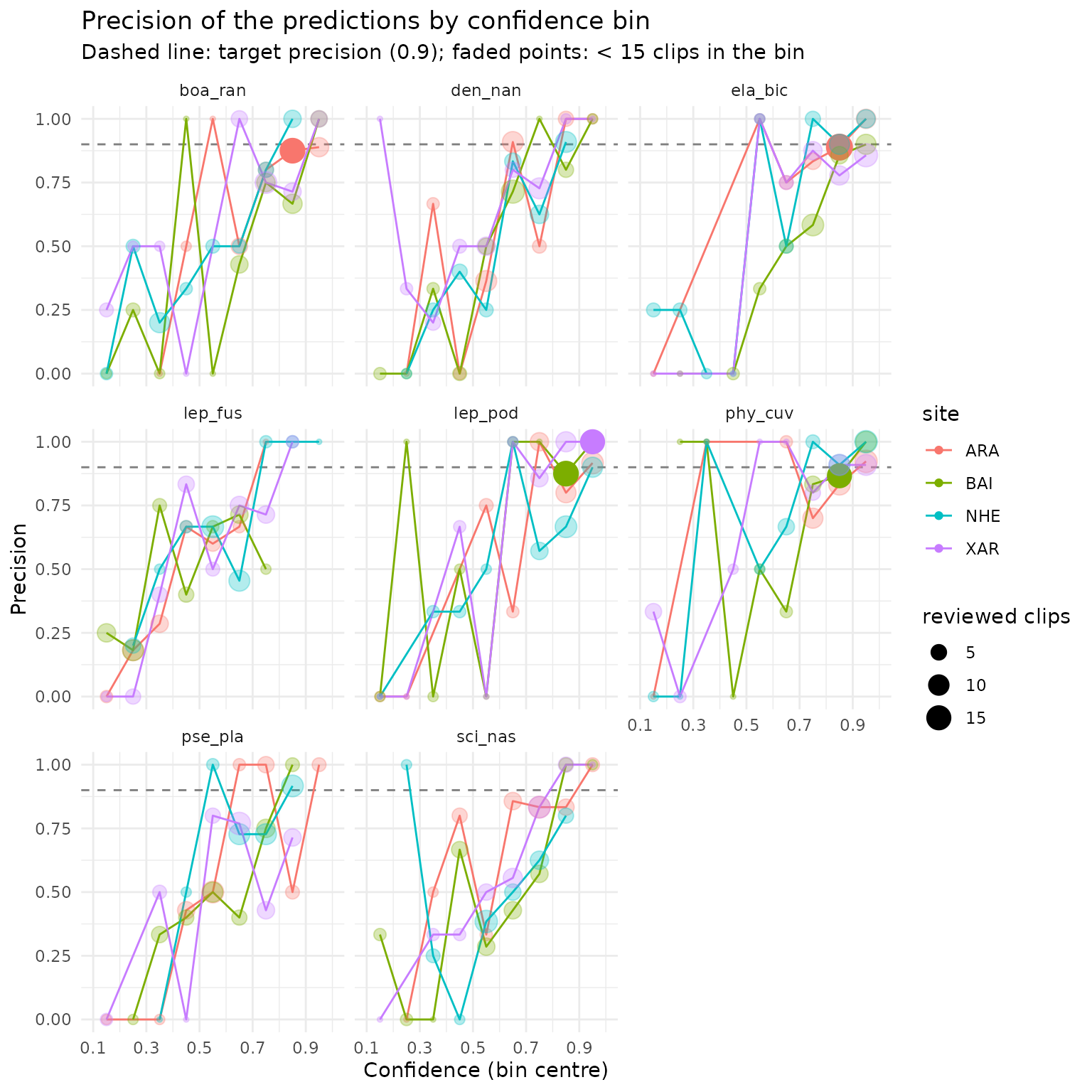
retraining_clips() lists the positive clips for
retraining the classifier. With real data,
post_validation() runs all of the above in one call and
writes each table to a CSV file, together with the figure.
Where next
-
vignette("sampling-designs"): choosing between the"top","random_detections"and"random_recordings"designs, the inclusion probabilities they record, and limits on the review effort. -
vignette("validation-effort"): how many clips to validate, from the curve ofcalibration_effort()and the support of each site x species cell inprecision_by_bin()andsuggest_thresholds(). -
vignette("calibration"): calibrating confidence scores (stage 2): the candidate models, their cross-validated comparison, calibration curves, scoring of every detection and nightly detection histories (p_min, k). -
vignette("community-matrices"): from calibrated detections to community analyses (stage 3):community_matrices(), thek_minrule, the effort filter and ordinations with ‘vegan’. -
vignette("retraining"): turning the reviewed clips into training folders for BirdNET-Analyzer, with an independent test set. -
vignette("crywolf-integration"): the clip manifest and validation tables as input to occupancy models with false positives. -
vignette("frognet-workflow"): the complete workflow as used in the FrogNet project.