False-positive rates that vary among sites and occasions • crywolf

The basic model has one false-positive rate for all sites and occasions, or a rate that depends on site covariates through fp = ~ .... Two other patterns are common in acoustic data. The rate can differ among sites for reasons nobody measured: a stream at one site, a frog chorus at another. And it can change from one occasion to the next with conditions that are measured on each recording, such as wind or rain noise. This article fits both patterns to simulated data whose truth is known, and compares the results with the constant-rate model.

The fitting code is shown but not run when the article is built; the results come from dev/precompute-fp-variation.R.

Unexplained variation among sites

The model

With random_fp = TRUE, the logit of the false-positive rate of site i gets a site effect,

\mathrm{logit}(p_{10,i}) = \gamma_0 + \mathbf{x}_i^\top \boldsymbol{\gamma} + e_i, \qquad e_i \sim \mathrm{Normal}(0, \sigma_{\mathrm{fp}}),

where \gamma_0 is the intercept of the rate, \mathbf{x}_i are the site covariates of fp (none here), and \sigma_{\mathrm{fp}}, reported as sd_fp_site, measures how much the rate varies among sites. Its prior is half-Normal with scale fp_priors()$fp_site_sd (1 by default). Each site effect is informed only by the automated detections of its own site, so with few occasions per site the estimates are pulled towards the mean.

The data

sim <- simulate_fp(nsite = 200, nocc = 10, sigma_p10 = 1, frac_verified = 0.3,
                   seed = 1)
m_const <- fp_occu(sim$data, occ = ~ x, fp = ~ 1, random_recorder = FALSE)
m_rand <- fp_occu(sim$data, occ = ~ x, fp = ~ 1, random_recorder = FALSE,
                  random_fp = TRUE)

The rate of each site is drawn on the logit scale around a base rate of 0.05 with a standard deviation of 1, which gives a mean rate over sites of 0.071. The true occupancy slope is -0.8.

Results

tab(list(constant = res$among$constant, random_fp = res$among$random),
    c("occ_x", "fp_(Intercept)", "p10_bar", "sd_fp_site"))
#>       model       variable   mean  lower  upper  rhat
#> 1  constant          occ_x -0.461 -0.775 -0.160 1.000
#> 2  constant fp_(Intercept) -2.880 -3.245 -2.545 1.000
#> 3  constant        p10_bar  0.054  0.037  0.073 1.000
#> 4 random_fp          occ_x -0.530 -0.874 -0.224 1.000
#> 5 random_fp fp_(Intercept) -3.066 -3.686 -2.524 1.003
#> 6 random_fp        p10_bar  0.098  0.053  0.151 1.010
#> 7 random_fp     sd_fp_site  1.559  0.755  2.336 1.005

The constant-rate model estimates the occupancy slope at -0.46 [-0.77, -0.16], which misses the true value of -0.8. With the site effect the estimate is -0.53 [-0.87, -0.22], still below the truth but with an interval that contains it, and the standard deviation of the site effects, 1.56 [0.75, 2.34], covers the true value of 1. Unexplained variation among sites is not harmless: in this dataset it pulled the occupancy slope towards zero, as sites with a high false-positive rate look occupied whatever their covariate. One dataset shows that it can happen; fp_calibrate() with sigma_p10 in the design measures how often.

fp_sites() gives the rate of each site, which with the site effect is a compromise between the site’s own data and the mean:

s <- res$among$random$sites
s$truth <- res$among$truth$p10_site
ggplot2::ggplot(s, ggplot2::aes(truth, p10)) +
  ggplot2::geom_abline(linetype = "dashed", colour = "grey50") +
  ggplot2::geom_point(alpha = 0.6, colour = "#241042") +
  ggplot2::scale_x_log10() + ggplot2::scale_y_log10() +
  ggplot2::labs(x = "True false-positive rate", y = "Estimated rate (posterior mean)") +
  ggplot2::theme_minimal()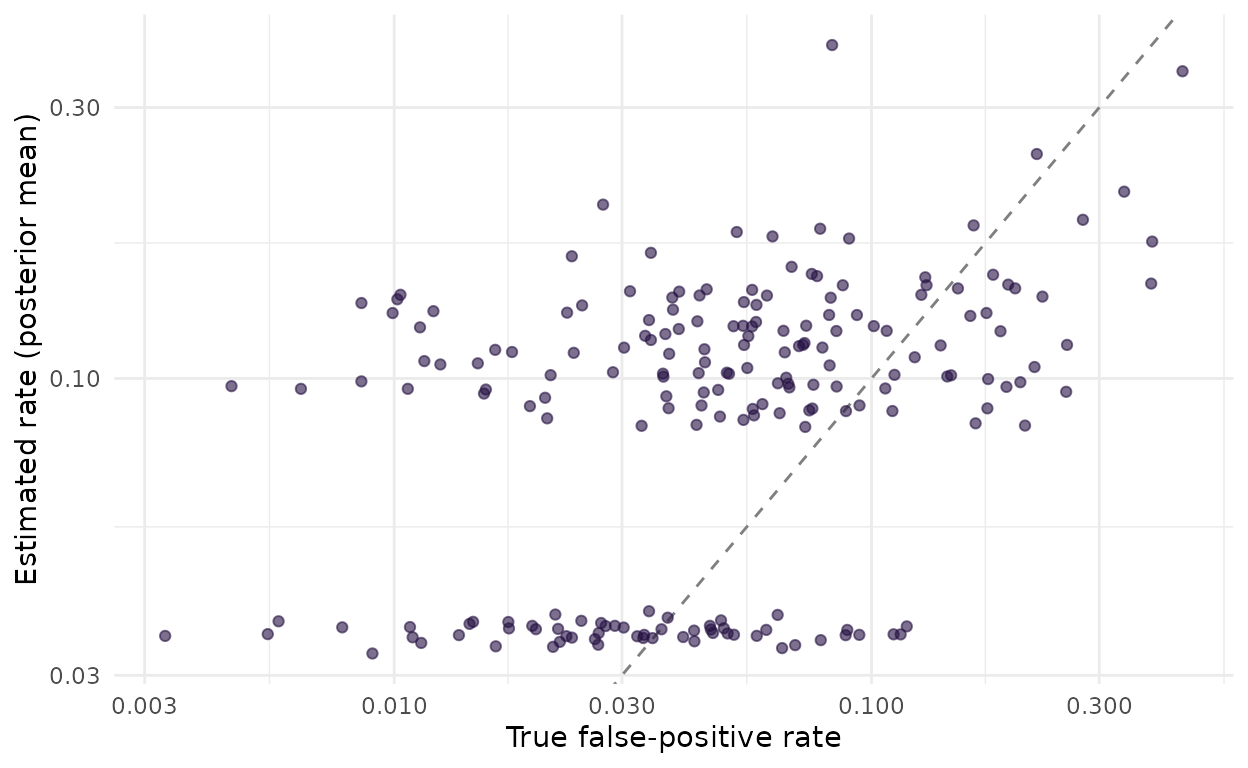

False-positive rate of each site estimated with the site effect against the true rate used in the simulation, on log scales. The dashed line marks equality.

The estimates fall into two groups. The 59 sites without any automated detection all get a low rate, between 0.033 and 0.039, whatever their true rate; the sites with detections get higher rates, which track the truth only loosely (correlation over all sites 0.45). Ten occasions per site say little about one site’s rate, and at a site that may be occupied a detection can be true or false. The site effect matters for the occupancy slope through the sites as a whole, not as a way to rank sites by their false-positive rate.

Costs and caveats

Mixing. The fit with the site effect took 27 seconds against 9 for the constant rate, and its smallest bulk effective sample size was 371 (largest R-hat 1.01). In 20 simulated datasets of the same kind with 300 sites and 20 occasions, 3 fits had an R-hat above 1.01 with the default settings (dev/profile/rejected-2026-10-21.md). Check the diagnostics, and run more iterations when they flag a problem.
Model comparison. Leaving a site out means its own effect is not known, so loo() integrates each site’s effect out of its log-likelihood (by Gauss-Hermite quadrature) before the leave-one-out computation. Conditional on the fitted effects, as in the log_lik of the Stan program, many sites would have Pareto k above 0.7; integrated, 0 do here. The difference in favour of the site effect is about 1.7 times its standard error, not a decisive one.

loo::loo_compare(list(constant = res$among$constant$loo,
                      random_fp = res$among$random$loo))
#>      model elpd_diff se_diff p_worse diag_diff diag_elpd
#>  random_fp       0.0     0.0      NA                    
#>   constant      -4.8     2.8    0.96

Confounding. The site effect is independent of the covariates by construction. It does not fix a false-positive rate that tracks the occupancy gradient: for that, model the rate on the covariates (vignette("crywolf")).

Variation among occasions

The model

A false-positive formula can use covariates of the automated table. The rate then varies among the occasions of a site:

\mathrm{logit}(p_{10,ik}) = \gamma_0 + \gamma_{\mathrm{noise}}\, \mathrm{noise}_{ik},

where \mathrm{noise}_{ik} is a measurement on occasion k of site i, standardized. The prior on \gamma_{\mathrm{noise}} is the slope prior of fp_priors(). Site and occasion covariates can be mixed in one formula.

The data

The data were simulated with a background-noise covariate, drawn at random for every occasion, that raises the logit of the false-positive rate by 1 per standard deviation, from a base rate of 0.05. In practice the covariate is a column of the automated table:

m_const <- fp_occu(d, occ = ~ x, fp = ~ 1, random_recorder = FALSE)
m_noise <- fp_occu(d, occ = ~ x, fp = ~ noise, random_recorder = FALSE)

Results

tab(list(constant = res$within$constant, noise = res$within$noise),
    c("occ_x", "fp_(Intercept)", "fp_noise", "p10_bar"))
#>      model       variable   mean  lower  upper  rhat
#> 1 constant          occ_x -0.788 -1.163 -0.441 1.001
#> 2 constant fp_(Intercept) -2.265 -2.537 -2.018 1.001
#> 3 constant        p10_bar  0.095  0.073  0.117 1.001
#> 4    noise          occ_x -0.751 -1.088 -0.438 1.001
#> 5    noise fp_(Intercept) -2.687 -3.041 -2.362 1.003
#> 6    noise       fp_noise  0.898  0.635  1.186 1.001
#> 7    noise        p10_bar  0.089  0.071  0.109 1.000

The noise effect is estimated at 0.90 [0.64, 1.19] (true value 1), and the mean rate over occasions at 0.089 [0.071, 0.109] (true value 0.076). Because the noise was drawn independently of the occupancy covariate, the constant-rate model still estimates the occupancy slope well, at -0.79 [-1.16, -0.44]. What it cannot do is say which detections are suspect: under the noise model, a detection in a noisy recording counts as weaker evidence of presence. LOO prefers the noise model clearly:

loo::loo_compare(list(constant = res$within$constant$loo,
                      noise = res$within$noise$loo))
#>     model elpd_diff se_diff p_worse diag_diff diag_elpd
#>     noise       0.0     0.0      NA                    
#>  constant     -25.1     7.5    1.00

If noise were correlated with the occupancy covariate, as when noisy sites are also those with less habitat, leaving it out would bias the slope as in vignette("calibration").

Which to use

A measured cause of false positives, at the site or the occasion level, belongs in the fp formula. It adds one coefficient per covariate rather than one effect per site, and modelling the measured cause is what restored calibrated intervals in the simulations of vignette("calibration") when the cause was correlated with occupancy.
random_fp = TRUE is for variation among sites that no covariate explains. It costs time and mixing. It is off by default.
With neither, the false-positive rate is assumed equal everywhere. A posterior predictive check (fp_ppc()) that flags sites with more detections than the model expects is a sign that this is wrong.