Introduction to crywolf • crywolf

Introduction

Automated detectors, such as the acoustic classifiers that scan thousands of hours of recordings (e.g. BirdNET; Kahl et al., 2021), make two kinds of mistakes. They miss calls of the target species (false negatives), and they label other sounds as the target species (false positives). Occupancy models deal with the first kind by repeating surveys at each site (MacKenzie et al., 2002), but they assume that every detection is real. Ignoring false positives inflates occupancy and, as we show below, can also distort the effect of environmental covariates on occupancy (Royle & Link, 2006).

crywolf fits the multiple-methods false-positive occupancy model of Miller et al. (2011) in a Bayesian framework, using Stan through the ‘cmdstanr’ interface. In this design, the automated method runs at every site, and a subset of its output, or a separate survey, is verified by an expert, so that some detections are known to be correct. The verified data tell the model how often the automated method is wrong. Chambert et al. (2015) and Clare et al. (2021) review this and other designs for false-positive error.

The package also simulates data under different false-positive regimes and checks, by simulation, whether the credible intervals of a model are calibrated for a given design. The simulation study behind the package (Provete et al., in preparation) showed that a constant false-positive rate gives well-calibrated intervals for the occupancy slope when false positives are homogeneous across sites. Random variation of the rate among sites made the estimate of the rate itself unreliable, but largely spared the occupancy slope (coverage of 0.81, against the nominal 0.95). When the rate tracked an environmental gradient correlated with the occupancy covariate, and the confusion was strong, the occupancy slope was biased towards zero and its intervals rarely contained the true value, and verifying up to 90% of the sites did not fix it. Letting the false-positive rate depend on covariates did. Weak confusion left the constant-rate model calibrated.

This vignette walks through a complete analysis with simulated data:

assembling data with fp_data() and simulate_fp();
the model, its priors, and how to change them with fp_priors();
fitting models with fp_occu(), with a constant false-positive rate and with a rate that depends on site covariates;
convergence diagnostics and posterior predictive checks with fp_ppc();
model comparison with leave-one-site-out cross-validation, and prediction (see ?fp_occu-methods);
detection covariates and recorder random effects;
the observation-confirmation design of Chambert et al. (2015), in which an expert checks the observations of some automated occasions.

fp_calibrate(), which checks the calibration of a model for your own design, has its own vignette, vignette("calibration", package = "crywolf").

Installation

crywolf fits its models with CmdStan through ‘cmdstanr’, which is not on CRAN. Install the package and ‘cmdstanr’ from R-universe, then CmdStan once:

install.packages("crywolf", repos = c("https://diogoprov.r-universe.dev",
                                      "https://stan-dev.r-universe.dev",
                                      getOption("repos")))
cmdstanr::install_cmdstan()

We load the package, together with ‘ggplot2’ and ‘bayesplot’ for the figures, and set a seed so that the results can be reproduced.

library(crywolf)
library(ggplot2)
library(bayesplot)
#> This is bayesplot version 1.16.0
#> - Online documentation and vignettes at mc-stan.org/bayesplot
#> - bayesplot theme set to bayesplot::theme_default()
#>    * Does _not_ affect other ggplot2 plots
#>    * See ?bayesplot_theme_set for details on theme setting
set.seed(2026)

Example data

The multiple-methods design

Each site i is surveyed K_i times by the automated method, for example K_i recordings scanned by a classifier. These are the automated occasions; each gives a detection (y_{ik} = 1) or not (y_{ik} = 0), and a detection may be a false positive. At a subset of sites, an expert also checks M_i occasions, for example by listening to clips. These are the verified occasions (v_{im}). A verified detection is certain: the species was there.

Simulated data

We simulate 300 sites with 20 automated occasions each, of which about 30% are verified on three occasions. Occupancy declines along a standardized covariate x (true slope -0.8). False positives are rare on average (baseline rate 0.05), but they increase along a second gradient, w, whose correlation with x is 0.7. This is what happens, for instance, when a soundalike species becomes more common where the target is rare. In real data, w is usually not measured; simulate_fp() returns it so that we can fit the true model as a positive control.

sim <- simulate_fp(nsite = 300, nocc = 20, psi = 0.5, b1 = -0.8,
                   p11 = 0.6, p10 = 0.05,
                   conf_effect = 1.5, conf_cor = 0.7,
                   frac_verified = 0.3, seed = 2026)
sim$data
#> <fp_data>
#>   sites:                  300
#>   automated occasions:    6000 (naive occupancy 0.87)
#>   verified sites:         85 (255 occasions, 39 with a confirmed detection)
#>   recorders:              5
#>   site covariates:        x, w 
#>   observation covariates: bio, aci

The data object holds three tables in long format, one row per occasion: the automated detections (auto, with two observation covariates and a recorder identifier), the verified detections (verified), and the sites with their covariates (sites).

head(sim$data$auto)
#>   site occasion y        bio         aci recorder
#> 1    1        1 0 -1.3818134 -0.36543963        5
#> 2    2        1 1  0.4355887  1.57117657        5
#> 3    3        1 0  0.3721785 -2.45643384        4
#> 4    4        1 0 -0.7030971  1.26171428        5
#> 5    5        1 1 -1.0114298 -1.02790936        4
#> 6    6        1 1 -1.6309700 -0.06734317        5
head(sim$data$verified)
#>    site occasion y
#> 3     3        1 0
#> 4     4        1 0
#> 5     5        1 1
#> 9     9        1 0
#> 11   11        1 1
#> 14   14        1 0
head(sim$data$sites)
#>   site          x           w
#> 1    1  0.5035356  0.40752869
#> 2    2 -1.1789366 -0.01491001
#> 3    3  0.1025980  0.66579653
#> 4    4 -0.1328932 -0.22992891
#> 5    5 -0.7446706 -1.44037323
#> 6    6 -2.6891101 -3.06909421

The element truth holds the generating values. Because the false-positive rate depends on w, it varies among sites: its mean over sites is 0.106, about twice the baseline, and it is highest where the target is least likely to occur.

p10_sites <- sim$data$sites
p10_sites$p10 <- sim$truth$p10_site
ggplot(p10_sites, aes(x, p10, colour = w)) +
  geom_point(alpha = 0.8) +
  scale_colour_viridis_c() +
  labs(x = "Occupancy covariate (x)",
       y = "False-positive rate (p10)", colour = "w") +
  theme_minimal()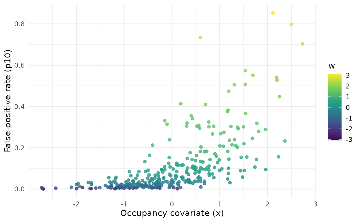

True false-positive rate at each site against the occupancy covariate x, coloured by the confusing gradient w.

Your own data

fp_data() builds the same object from your own tables. Each needs a site column and a 0/1 detection column; covariates are taken from sites (for occupancy and false positives) and from auto (for true detection). Sites may differ in the number of occasions.

auto <- data.frame(
  site = rep(c("A", "B", "C"), times = c(3, 2, 3)),
  y    = c(1, 0, 1,  0, 0,  1, 1, 0),
  wind = c(0.2, -0.5, 1.1, 0.3, -1.4, 0.8, 0.0, -0.6)
)
verified <- data.frame(site = c("A", "A", "C"), y = c(1, 0, 0))
sites <- data.frame(site = c("A", "B", "C"), forest = c(0.4, -1.2, 0.8))
fp_data(auto, sites, verified)
#> <fp_data>
#>   sites:                  3
#>   automated occasions:    8 (naive occupancy 0.67)
#>   verified sites:         2 (3 occasions, 1 with a confirmed detection)
#>   site covariates:        forest 
#>   observation covariates: wind

Site A has a verified detection, so it is known to be occupied. If your detections are stored as site-by-occasion matrices, as in ‘unmarked’, use fp_data_wide() instead.

The multiple-methods false-positive occupancy model

Basic model description

Let z_i be the true occupancy state of site i (z_i = 1 if the species is present). We model it as

z_i \sim \text{Bernoulli}(\psi_i), \qquad \text{logit}(\psi_i) = \mathbf{x}_i^\top \boldsymbol{\beta},

where \psi_i is the occupancy probability, \mathbf{x}_i is the vector of site covariates (with a leading 1 for the intercept), and \boldsymbol{\beta} the vector of occupancy coefficients.

A detection by the automated method on occasion k can come from an occupied site (a true detection, with probability p_{11,ik}) or from an unoccupied site (a false positive, with probability p_{10,i}):

y_{ik} \mid z_i \sim \text{Bernoulli}\left(z_i\, p_{11,ik} + (1 - z_i)\, p_{10,i}\right).

The true-detection probability depends on observation covariates \mathbf{d}_{ik} (e.g. background noise on that recording) and, optionally, on a random intercept u_{r} for the recorder r used at the site:

\text{logit}(p_{11,ik}) = \mathbf{d}_{ik}^\top \boldsymbol{\alpha} + u_{r[i]}, \qquad u_r \sim \text{Normal}(0, \sigma_u^2),

where the first element of \boldsymbol{\alpha}, \alpha_0, is the intercept. The false-positive rate depends on site covariates \mathbf{f}_i:

\text{logit}(p_{10,i}) = \gamma_0 + \mathbf{f}_i^\top \boldsymbol{\gamma}, \qquad \gamma_0 = \alpha_0 - \Delta, \quad \Delta > 0.

With no covariates in \mathbf{f}_i, the rate is constant across sites.

The verified method cannot produce false positives. Its detection probability is r_{11}:

v_{im} \mid z_i \sim \text{Bernoulli}(z_i\, r_{11}), \qquad \text{logit}(r_{11}) = \delta_0.

The gap \Delta. Without further constraints, the model has two equivalent solutions: one in which occupied sites are those with many detections, and one in which the labels of the two states are swapped. We write the false-positive intercept as the true-detection intercept minus a positive gap, \Delta, so that at the reference values of the covariates (all zero) a true detection is always more likely than a false positive. This removes the label switching. Because the reference is the point where all covariates are zero, centre or standardize them, so that the constraint applies at an average site.

The role of the verified data. A site with at least one verified detection is known to be occupied. Verified data at occupied and unoccupied sites separate the two sources of automated detections and anchor p_{10}. Without any verified data the false-positive rate is informed only by the priors and the gap, and fp_occu() warns about it.

Likelihood. The latent state z_i is summed out, so the likelihood of site i is

\begin{aligned} L_i ={}& \psi_i \prod_{k} p_{11,ik}^{y_{ik}} (1 - p_{11,ik})^{1 - y_{ik}} \prod_{m} r_{11}^{v_{im}} (1 - r_{11})^{1 - v_{im}} \\ &+ (1 - \psi_i) \prod_{k} p_{10,i}^{y_{ik}} (1 - p_{10,i})^{1 - y_{ik}} \prod_{m} (1 - v_{im}), \end{aligned}

where the last product is zero at sites with a verified detection and one elsewhere. Summing out z_i makes sampling efficient in Stan and gives one log-likelihood value per site, which we use for cross-validation below. The Stan program itself is in the file returned by fp_stan_file().

The model as a graph. The directed acyclic graph below shows how the pieces fit together, from the priors (top) to the data (bottom). The automated detections y_{ik} appear as y^{aut}_{ik} and the verified detections v_{im} as y^{ver}_{im}. Both depend on the latent state z_i, which is why the verified data, through z_i, inform the false-positive rate.

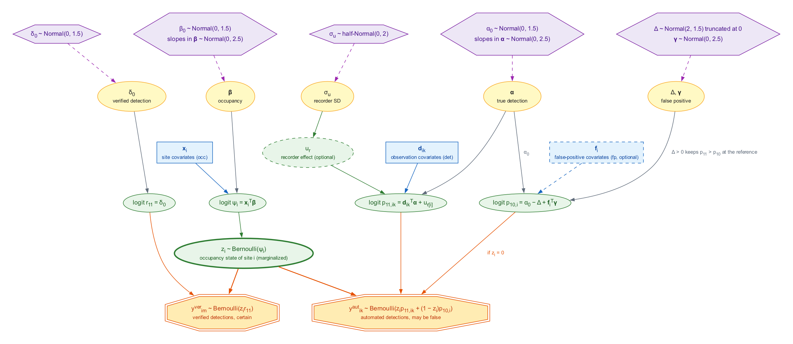
Directed acyclic graph of the multiple-methods false-positive occupancy model fitted by fp_occu(). Hexagons are priors (defaults of fp_priors()), yellow ellipses are parameters, blue boxes are covariates, green ellipses are latent quantities and linear predictors, and octagons are the observed data. Dashed outlines mark optional components: false-positive covariates (fp = ~ ...) and the recorder random intercept (random_recorder = TRUE). Adapted from the fpcalib research compendium.

Priors

All parameters have explicit priors on the logit scale, which are weakly informative when covariates are standardized:

Parameter	Prior (default)	Argument of `fp_priors()`
Intercepts \beta_0, \alpha_0, \delta_0	\text{Normal}(0, 1.5)	`intercept_sd`
Slopes in \boldsymbol{\beta}, \boldsymbol{\alpha}, \boldsymbol{\gamma}	\text{Normal}(0, 2.5)	`slope_sd`
Gap \Delta	\text{Normal}(2, 1.5), truncated at 0	`gap_mean`, `gap_sd`
Recorder SD \sigma_u	\text{half-Normal}(0, 2)	`recorder_sd`

A Normal(0, 1.5) prior on an intercept is roughly flat on the probability scale between 0.05 and 0.95. The prior on \Delta places the false-positive rate at the reference about an order of magnitude below true detection, while leaving room for the data to move it. fp_priors() prints the settings and lets you change them:

fp_priors()
#> <fp_priors> (logit scale)
#>   intercepts      ~ Normal(0, 1.5)
#>   slopes          ~ Normal(0, 2.5)
#>   fp_gap          ~ Normal(2, 1.5), truncated at 0
#>   sd_recorder     ~ half-Normal(0, 2)
#>   sd_fp_site      ~ half-Normal(0, 1)
fp_priors(slope_sd = 1, gap_sd = 1)
#> <fp_priors> (logit scale)
#>   intercepts      ~ Normal(0, 1.5)
#>   slopes          ~ Normal(0, 1)
#>   fp_gap          ~ Normal(2, 1), truncated at 0
#>   sd_recorder     ~ half-Normal(0, 2)
#>   sd_fp_site      ~ half-Normal(0, 1)

Parameter names

The output labels each coefficient by its process and by the column of the design matrix it multiplies:

Symbol	Output name
\boldsymbol{\beta}	`occ_(Intercept)`, `occ_x`, …
\boldsymbol{\alpha}	`det_(Intercept)`, `det_bio`, …
\gamma_0, \boldsymbol{\gamma}	`fp_(Intercept)`, `fp_w`, …
\Delta	`fp_gap`
\delta_0, r_{11}	`verified_(Intercept)`, `p_verified`
\sigma_u	`sd_recorder`
p_{11}, p_{10} at the reference	`p11_ref`, `p10_ref`
mean of p_{10,i} over the sites	`p10_bar`

Fitting the constant-rate model with fp_occu()

fp_occu() takes one formula for each process: occ for occupancy, det for true detection, and fp for the false-positive rate. With fp = ~ 1 the rate is constant across sites, which is what most applications assume. random_recorder adds the recorder random intercept; the simulated data include a recorder column, but recorders have no effect in this simulation, so we turn it off. The sampler runs four chains of 1000 warm-up and 1000 sampling iterations by default (chains, iter_warmup, iter_sampling), with a target acceptance rate adapt_delta = 0.95; other arguments are passed to the $sample() method of ‘cmdstanr’. With many sites or occasions, threads_per_chain lets each chain use several cores (see vignette("stan_model", package = "crywolf")). The model is compiled the first time it is used and cached for later sessions.

m_const <- fp_occu(sim$data, occ = ~ x, det = ~ 1, fp = ~ 1,
                   random_recorder = FALSE, seed = 1)
m_const
#> Bayesian false-positive occupancy model (multiple-methods design)
#> 
#>   occupancy:       ~x 
#>   true detection:  ~1  
#>   false positive:  ~1  
#>   data:            300 sites, 6000 automated and 255 verified occasions
#> 
#>              variable    mean      sd   lower   upper rhat ess_bulk ess_tail
#>       occ_(Intercept)  0.4395 0.12287  0.1944  0.6848    1     4101     2670
#>                 occ_x -0.2565 0.12348 -0.5015 -0.0187    1     4382     2865
#>       det_(Intercept)  0.3506 0.03659  0.2801  0.4239    1     4323     2849
#>  verified_(Intercept) -0.0354 0.17185 -0.3663  0.2925    1     4526     2654
#>            p_verified  0.4912 0.04266  0.4094  0.5726    1     4526     2654
#>               p11_ref  0.5867 0.00887  0.5696  0.6044    1     4323     2849
#>        fp_(Intercept) -2.3946 0.09202 -2.5761 -2.2176    1     4425     2556
#>                fp_gap  2.7452 0.09055  2.5707  2.9225    1     4359     2649
#>               p10_ref  0.0839 0.00706  0.0707  0.0982    1     4425     2556
#>               p10_bar  0.0839 0.00706  0.0707  0.0982    1     4425     2556
#> 
#>   Sampler: 0 divergent transitions, max R-hat 1.004, min bulk/tail ESS 4101/2556

The printed table gives, for each parameter, the posterior mean, standard deviation, the limits of the 95% equal-tailed credible interval, and the convergence diagnostics discussed in the next section. The true-detection probability at the reference, p11_ref, and the probability of detection by the verified method, p_verified, are on the probability scale; the other coefficients are on the logit scale.

Convergence and model adequacy

Before interpreting any estimate, we check that the chains converged and that the model reproduces the data. These steps, together with the model comparison and the simulation-based checks of vignette("calibration", package = "crywolf"), follow the Bayesian workflow described by Gelman et al. (2026).

Convergence

fp_occu() reports, for every parameter, the rank-normalized \hat{R} (rhat) and the bulk and tail effective sample sizes (ess_bulk, ess_tail), and summarizes the sampler diagnostics in the last line of the output: the number of divergent transitions, the largest \hat{R}, and the smallest effective sample sizes. It warns when there are divergent transitions, when \hat{R} > 1.01, or when the bulk ESS is below 400. In this fit there were 0 divergent transitions, the largest \hat{R} was 1.004, and the smallest bulk ESS was 4101, so the chains mixed well. summary() returns the same table, with an adjustable interval width:

summary(m_const, prob = 0.9)
#> Posterior summary (90% equal-tailed intervals)
#> 
#>              variable    mean      sd   lower   upper rhat ess_bulk ess_tail
#>       occ_(Intercept)  0.4395 0.12287  0.2384  0.6437    1     4101     2670
#>                 occ_x -0.2565 0.12348 -0.4592 -0.0564    1     4382     2865
#>       det_(Intercept)  0.3506 0.03659  0.2898  0.4114    1     4323     2849
#>  verified_(Intercept) -0.0354 0.17185 -0.3199  0.2411    1     4526     2654
#>            p_verified  0.4912 0.04266  0.4207  0.5600    1     4526     2654
#>               p11_ref  0.5867 0.00887  0.5719  0.6014    1     4323     2849
#>        fp_(Intercept) -2.3946 0.09202 -2.5465 -2.2425    1     4425     2556
#>                fp_gap  2.7452 0.09055  2.5965  2.8957    1     4359     2649
#>               p10_ref  0.0839 0.00706  0.0727  0.0960    1     4425     2556
#>               p10_bar  0.0839 0.00706  0.0727  0.0960    1     4425     2556
#> 
#>   Sampler: 0 divergent transitions, max R-hat 1.004, min bulk/tail ESS 4101/2556

Trace plots show whether the chains explored the same region of the posterior. as_draws_df() returns the draws with readable names, which ‘bayesplot’ can plot directly:

draws_const <- as_draws_df(m_const)
color_scheme_set("purple")
mcmc_trace(draws_const, pars = c("occ_x", "fp_gap"))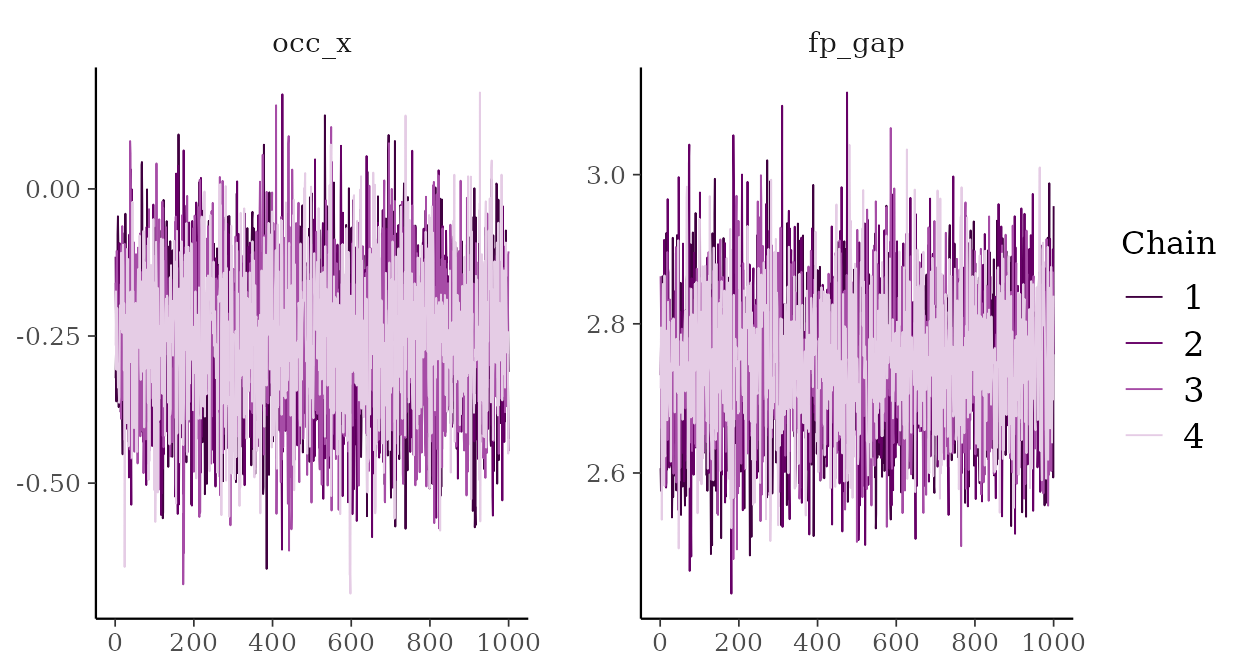

Trace plots of the occupancy slope and of the gap between the true-detection and false-positive intercepts, for the four chains.

Posterior predictive check

A posterior predictive check compares the observed data with data replicated from the fitted model (Gabry et al., 2019). fp_ppc() does this for the number of detections at each site. For each posterior draw, it draws the occupancy state of each site from its conditional posterior, replicates the detections, and computes a discrepancy statistic (by default, Freeman-Tukey) for the observed and the replicated data. The Bayesian p-value is the proportion of draws in which the replicated discrepancy exceeds the observed one; values near 0 or 1 indicate lack of fit.

ppc_const <- fp_ppc(m_const, seed = 1)
ppc_const
#> Posterior predictive check (automated detections per site)
#> 
#>   statistic:          freeman-tukey
#>   draws, sites:       1000, 300
#>   mean discrepancy:   observed 116, replicated 67
#>   Bayesian p-value:   0
#> 
#>   The p-value is far from 0.5: the model may not fit these data.

The elements y and yrep follow the conventions of ‘bayesplot’, so its ppc_*() functions work directly. Here we compare the distribution of the number of detections per site in the observed and replicated data:

ppc_bars(ppc_const$y, ppc_const$yrep) +
  labs(x = "Automated detections per site", y = "Number of sites")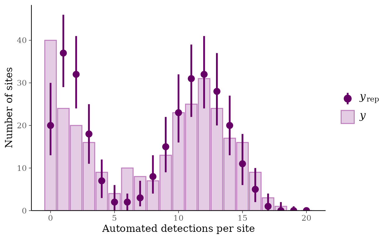

Posterior predictive check of the constant-rate model: number of sites with each number of automated detections, observed (bars) and replicated (points and intervals).

The Bayesian p-value of the constant-rate model is 0.00. The check flags a lack of fit: the model does not reproduce how detections are distributed among sites. In the figure, the replicated data have too few sites with no detections and too many with one or two, which is what we expect when the false-positive rate is in fact low at some sites and high at others. The next section shows why this matters.

Modelling the false-positive rate

Why the occupancy slope is biased

The true occupancy slope is -0.8. The constant-rate model estimates it at -0.26:

coef(m_const, "occ")
#> occ_(Intercept)           occ_x 
#>       0.4395490      -0.2564532

False positives in these data increase along w, which is correlated with x. A model that assumes a constant false-positive rate cannot attribute the extra detections at sites with high w to false positives, so it attributes part of them to occupancy. Sites where the classifier is fooled most look like sites where the species is present, and the occupancy slope is pulled towards zero. In the simulation study behind this package, verifying more sites did not remove this bias: verification anchors the mean false-positive rate, but not its dependence on the covariate, so a constant-rate model passes that dependence on to the occupancy slope however precisely the mean is estimated (Provete et al., in preparation).

A false-positive rate that tracks the occupancy covariate

The practical remedy is to let the false-positive rate depend on the occupancy covariate, which is always available:

m_x <- fp_occu(sim$data, occ = ~ x, det = ~ 1, fp = ~ x,
               random_recorder = FALSE, seed = 1)
coef(m_x, "fp")
#> fp_(Intercept)           fp_x 
#>      -2.656303       1.010679

The coefficient fp_x captures the part of the confusion that is correlated with x. In the simulation study, this model reduced the bias of the occupancy slope by 34 to 62% when the confusing gradient had a correlation of 0.7 with the occupancy covariate, and its intervals became better calibrated as more sites were verified, although coverage remained below the nominal level. When false positives depended on the occupancy covariate exactly, this model was fully calibrated (Provete et al., in preparation).

A false-positive rate that tracks the confusing gradient

If you have measured something that drives the confusion, such as the abundance of a soundalike species or an index of background noise, put it in the fp formula. In a simulation we know the confusing gradient w, so we can fit the generating model as a positive control:

m_w <- fp_occu(sim$data, occ = ~ x, det = ~ 1, fp = ~ w,
               random_recorder = FALSE, seed = 1)
summary(m_w)
#> Posterior summary (95% equal-tailed intervals)
#> 
#>              variable    mean      sd    lower   upper rhat ess_bulk ess_tail
#>       occ_(Intercept)  0.1077 0.12397 -0.13277  0.3485    1     5453     2996
#>                 occ_x -0.7825 0.14688 -1.08259 -0.5007    1     4412     2968
#>       det_(Intercept)  0.4332 0.03736  0.36147  0.5092    1     5045     2995
#>  verified_(Intercept)  0.3548 0.18982 -0.00476  0.7218    1     5385     2945
#>            p_verified  0.5870 0.04566  0.49881  0.6730    1     5385     2945
#>               p11_ref  0.6066 0.00891  0.58940  0.6246    1     5045     2995
#>        fp_(Intercept) -2.9022 0.09837 -3.10058 -2.7132    1     3722     3373
#>                  fp_w  1.4716 0.07567  1.32664  1.6230    1     3545     3002
#>                fp_gap  3.3354 0.10464  3.13681  3.5428    1     3472     3007
#>               p10_ref  0.0523 0.00486  0.04308  0.0622    1     3722     3373
#>               p10_bar  0.1073 0.00462  0.09836  0.1167    1     4904     3049
#> 
#>   Sampler: 0 divergent transitions, max R-hat 1.003, min bulk/tail ESS 3472/2945

The estimated effect of w on the false-positive rate is 1.47 (true value 1.5). Measured covariates are rarely the confusing gradient itself. In the simulation study, a proxy of the gradient (correlation 0.7 with w, related to x only through w) recovered less than the occupancy covariate did, reducing the bias of the slope by 17 to 37%. Only the part of the gradient aligned with the occupancy covariate distorts its slope, and the occupancy covariate captures that part by construction. The recommendation is therefore to include the occupancy covariates in fp, add any measured correlate of the confusion, and verify enough sites to tell the effects apart (Provete et al., in preparation).

The figure compares the occupancy slope of the three models with its true value.

slopes <- list(`fp = ~ 1` = m_const, `fp = ~ x` = m_x, `fp = ~ w` = m_w) |>
  purrr::imap(function(m, nm) {
    tab <- summary(m)$table
    data.frame(model = nm, tab[tab$variable == "occ_x", c("mean", "lower", "upper")])
  }) |>
  purrr::list_rbind()
slopes$model <- factor(slopes$model, levels = rev(slopes$model))
ggplot(slopes, aes(mean, model)) +
  geom_vline(xintercept = -0.8, linetype = "dashed") +
  geom_pointrange(aes(xmin = lower, xmax = upper), colour = "#5B2A86") +
  labs(x = "Occupancy slope on x", y = NULL) +
  theme_minimal()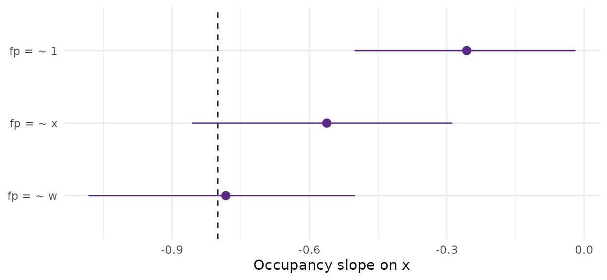

Posterior mean and 95% credible interval of the occupancy slope under three models of the false-positive rate. The dashed line marks the true value.

The posterior predictive checks of the three models agree with this picture:

list(`fp = ~ 1` = ppc_const, `fp = ~ x` = fp_ppc(m_x, seed = 1),
     `fp = ~ w` = fp_ppc(m_w, seed = 1)) |>
  purrr::map_dbl("p_value")
#> fp = ~ 1 fp = ~ x fp = ~ w 
#>    0.000    0.000    0.831

Only the model with the confusing gradient has a p-value far from 0. A posterior predictive check is a useful warning, but a p-value near 0.5 does not show that the false-positive process is correctly specified: with fewer occasions or weaker confusion, a misspecified model may pass the check and still have a biased slope. To ask whether the intervals of a model are calibrated for your design, use fp_calibrate() (see vignette("calibration", package = "crywolf")).

Sensitivity to the priors

To check that the conclusions do not depend on the priors, we refit the model with fp = ~ w using narrower priors on the slopes and on the gap, and compare the main parameters:

m_w_narrow <- fp_occu(sim$data, occ = ~ x, det = ~ 1, fp = ~ w,
                      random_recorder = FALSE, seed = 1,
                      priors = fp_priors(slope_sd = 1, gap_sd = 1))
pars <- c("occ_x", "fp_w", "fp_gap")
data.frame(parameter = pars,
           default = round(coef(m_w)[pars], 3),
           narrow  = round(coef(m_w_narrow)[pars], 3), row.names = NULL)
#>   parameter default narrow
#> 1     occ_x  -0.783 -0.770
#> 2      fp_w   1.472  1.459
#> 3    fp_gap   3.335  3.317

With 300 sites, the data dominate the priors and the estimates barely change. With smaller data sets, the priors, particularly the one on \Delta, matter more, and this comparison is worth reporting.

Variation that the covariates do not explain

The false-positive rate can also vary among sites for reasons that no measured covariate captures, for instance because some recorders sit near a noise source that the classifier confuses with the target. random_fp = TRUE adds a site random intercept to the logit of the rate, \text{logit}(p_{10,i}) = \gamma_0 + \mathbf{f}_i^\top \boldsymbol{\gamma} + e_i with e_i \sim \text{Normal}(0, \sigma_{fp}), and reports \sigma_{fp} as sd_fp_site:

m_re <- fp_occu(sim$data, occ = ~ x, fp = ~ x, random_recorder = FALSE,
                random_fp = TRUE, seed = 1)

The random effect is off by default because it is costly: it adds one parameter per site, fits take several times longer, and its chains mix less well, so check the diagnostics and run longer chains when needed. It recovers the mean false-positive rate when the rate varies at random among sites, but it does not correct false positives that follow the occupancy gradient, as in the data above; for those, the remedy is the covariates in fp. Use covariates first, and the random effect for the variation that remains. ?fp_occu gives the details.

Model comparison with LOO

Because the latent state is summed out, the pointwise log-likelihood is computed per site, and loo() gives approximate leave-one-site-out cross-validation by Pareto-smoothed importance sampling (Vehtari et al., 2017). loo_compare() ranks the models by their expected log predictive density (elpd):

loo_const <- loo(m_const)
loo_x <- loo(m_x)
loo_w <- loo(m_w)
loo::loo_compare(list(`fp = ~ 1` = loo_const, `fp = ~ x` = loo_x,
                      `fp = ~ w` = loo_w))
#>     model elpd_diff se_diff p_worse diag_diff diag_elpd
#>  fp = ~ w       0.0     0.0      NA                    
#>  fp = ~ x     -89.8    15.9    1.00                    
#>  fp = ~ 1    -135.8    18.2    1.00

The first row is the best model; elpd_diff is the difference in elpd from it, with its standard error se_diff. Here the model with the confusing gradient predicts best, followed by the model with fp = ~ x, and the constant-rate model predicts worst; the differences are several times their standard errors. Check the Pareto k diagnostics printed by loo(): values above 0.7 mean that the approximation is unreliable for those sites.

loo_w
#> Computed from 4000 by 300 log-likelihood matrix.
#> 
#>          Estimate    SE
#> elpd_loo  -3309.8  85.1
#> p_loo         5.6   0.4
#> looic      6619.7 170.2
#> ------
#> MCSE of elpd_loo is 0.0.
#> MCSE and ESS estimates assume independent draws (r_eff=1).
#> 
#> All Pareto k estimates are good (k < 0.7).
#> See help('pareto-k-diagnostic') for details.

LOO measures predictive performance, not the bias of a particular coefficient. It can tell which model of the false-positive rate fits better, but not whether the occupancy slope of the best model is unbiased.

Prediction

predict() returns the posterior mean and credible interval of the occupancy probability (process = "occ") or of the false-positive rate (process = "fp") for new values of the covariates. With summary = FALSE it returns the matrix of posterior draws instead, with one row per draw.

nd <- data.frame(x = seq(-2, 2, by = 1))
predict(m_x, newdata = nd, process = "occ")
#>    x  estimate     lower     upper
#> 1 -2 0.8007148 0.6936194 0.8863740
#> 2 -1 0.7006876 0.6213420 0.7755722
#> 3  0 0.5730807 0.5118715 0.6309239
#> 4  1 0.4343703 0.3411549 0.5272494
#> 5  2 0.3080732 0.1860316 0.4478089
predict(m_x, newdata = nd, process = "fp")
#>    x    estimate       lower      upper
#> 1 -2 0.009539925 0.005490955 0.01538964
#> 2 -1 0.025280477 0.017684257 0.03471712
#> 3  0 0.065871816 0.054122079 0.07819775
#> 4  1 0.162054380 0.139157832 0.18558329
#> 5  2 0.347229508 0.278738876 0.41289238

Predicting over a grid of the occupancy covariate shows how the bias of the slope translates into the occupancy probability:

grid <- data.frame(x = seq(-2.5, 2.5, length.out = 50))
pred <- list(`fp = ~ 1` = m_const, `fp = ~ x` = m_x, `fp = ~ w` = m_w) |>
  purrr::imap(function(m, nm) {
    data.frame(model = nm, predict(m, newdata = grid, process = "occ"))
  }) |>
  purrr::list_rbind()
truth <- data.frame(x = grid$x, psi = plogis(sim$truth$b0 + sim$truth$b1 * grid$x))
ggplot(pred, aes(x, estimate)) +
  geom_ribbon(aes(ymin = lower, ymax = upper, fill = model), alpha = 0.2) +
  geom_line(aes(colour = model)) +
  geom_line(aes(x, psi), data = truth, linetype = "dashed") +
  scale_colour_manual(values = c("#FF3EA5", "#2DE2E6", "#5B2A86")) +
  scale_fill_manual(values = c("#FF3EA5", "#2DE2E6", "#5B2A86")) +
  labs(x = "Occupancy covariate (x)", y = "Occupancy probability",
       colour = NULL, fill = NULL) +
  theme_minimal()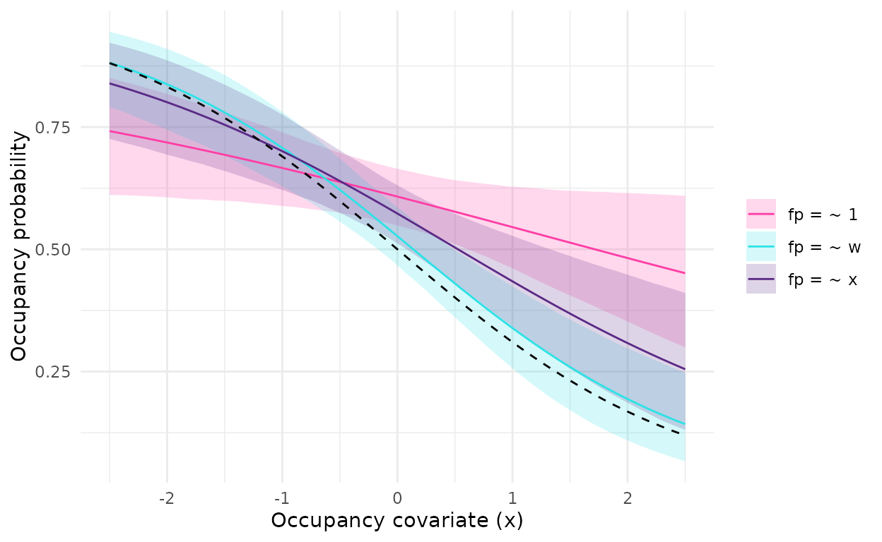

Predicted occupancy probability (posterior mean and 95% credible interval) along the occupancy covariate under three models of the false-positive rate. The dashed line is the true relationship.

Detection covariates and recorder effects

The true-detection formula accepts observation covariates (columns of auto, which may change from occasion to occasion) and site covariates. With random_recorder = TRUE, the model adds a random intercept for each recorder, which absorbs differences in sensitivity among devices or observers. Name the recorder column with the recorder argument of fp_data().

We simulate a second data set in which two acoustic indices, bio and aci, affect true detection (effects 0.5 and -0.3), and ten recorders differ in sensitivity (standard deviation 0.6 on the logit scale):

sim_rec <- simulate_fp(nsite = 300, nocc = 20, a_bio = 0.5, a_aci = -0.3,
                       sd_recorder = 0.6, nrec = 10,
                       conf_effect = 1.5, conf_cor = 0.7, seed = 2027)
m_rec <- fp_occu(sim_rec$data, occ = ~ x, det = ~ bio + aci, fp = ~ w,
                 random_recorder = TRUE, seed = 1)
m_rec

When detection covariates change among occasions, each occasion enters the likelihood separately, instead of being grouped with the other occasions of its site, so the model takes longer to fit (about a minute here). To keep this vignette quick to build, we show the saved output of this fit:

#> Bayesian false-positive occupancy model (multiple-methods design)
#> 
#>   occupancy:       ~x 
#>   true detection:  ~bio + aci + (1 | recorder) 
#>   false positive:  ~w 
#>   data:            300 sites, 6000 automated and 270 verified occasions
#> 
#>              variable    mean      sd   lower   upper rhat ess_bulk ess_tail
#>       occ_(Intercept) -0.0438 0.12139 -0.2903  0.1874    1     4009     2863
#>                 occ_x -0.6366 0.14009 -0.9196 -0.3665    1     4515     2761
#>       det_(Intercept)  0.2686 0.21205 -0.1726  0.6760    1      875     1188
#>               det_bio  0.4145 0.04293  0.3330  0.4976    1     4116     2652
#>               det_aci -0.3188 0.04106 -0.3987 -0.2382    1     4032     2650
#>  verified_(Intercept)  0.5614 0.17494  0.2173  0.9020    1     4265     3009
#>            p_verified  0.6358 0.04024  0.5541  0.7114    1     4265     3009
#>               p11_ref  0.5661 0.05151  0.4570  0.6628    1      875     1188
#>        fp_(Intercept) -2.9961 0.10328 -3.2001 -2.8032    1     4049     3336
#>                  fp_w  1.5605 0.09049  1.3917  1.7402    1     4023     2873
#>                fp_gap  3.2648 0.23471  2.7838  3.7208    1      990     1411
#>               p10_ref  0.0478 0.00468  0.0392  0.0572    1     4049     3336
#>               p10_bar  0.1003 0.00485  0.0909  0.1102    1     4174     3274
#>           sd_recorder  0.6284 0.18510  0.3736  1.0802    1      932     1796
#> 
#>   Sampler: 0 divergent transitions, max R-hat 1.003, min bulk/tail ESS 875/1188

The effects of the acoustic indices (det_bio, det_aci), the standard deviation among recorders (sd_recorder), and the effect of the confusing gradient (fp_w) are close to their true values. The true-detection intercept, the gap, and the recorder standard deviation have lower effective sample sizes than the other parameters, as is common with random intercepts, but all are above the threshold of 400.

The observation-confirmation design

In the design used so far, the verified method is separate from the automated one, and its detections identify occupied sites. In many acoustic studies, an expert instead listens to the clips that the classifier flagged and labels each one as the target species or not. Chambert et al. (2015) called this the observation-confirmation design. Each checked occasion ends in one of four states: nothing was assigned to the species (0), all assigned observations were false (1), all were true (2), or both kinds were found (3). Because false observations can now be seen directly, at occupied sites as well as at unoccupied ones, the model describes each occasion by two probabilities: s_1, of at least one true observation (at an occupied site), and s_0, of at least one false observation. The probabilities of the four states v = 0, 1, 2, 3 are

\begin{aligned} \Pr(v \mid z = 1) &= \bigl[(1 - s_1)(1 - s_0),\; (1 - s_1)\, s_0,\\ &\qquad s_1 (1 - s_0),\; s_1 s_0\bigr],\\ \Pr(v \mid z = 0) &= \bigl[1 - s_0,\; s_0,\; 0,\; 0\bigr], \end{aligned}

and an occasion that was not checked is a detection with probability p_{11} = 1 - (1 - s_1)(1 - s_0) at an occupied site and p_{10} = s_0 at an unoccupied one. The formulas det and fp of fp_occu() then model \text{logit}(s_1) and \text{logit}(s_0).

To use this design, add two columns to auto with the number of observations confirmed as the species and as something else, NA on the occasions that were not checked, and name them in the confirmed argument of fp_data(). All observations of a checked occasion must be checked. simulate_fp() generates such data with frac_confirmed, the probability that an occasion is checked:

sim_conf <- simulate_fp(nsite = 200, nocc = 10, p10 = 0.1,
                        frac_confirmed = 0.3, frac_verified = 0, seed = 2028)
sim_conf$data
#> <fp_data>
#>   sites:                  200
#>   automated occasions:    2000 (naive occupancy 0.83)
#>   verified sites:         0 (0 occasions, 83 with a confirmed detection)
#>   confirmed occasions:    640 (188 with a true observation)
#>   recorders:              5
#>   site covariates:        x, w 
#>   observation covariates: bio, aci
head(sim_conf$data$auto[!is.na(sim_conf$data$auto$n_true), ])
#>    site occasion y         bio        aci recorder n_true n_false
#> 8     8        1 1  1.12027961  0.1841090        3      1       1
#> 10   10        1 1  1.65371742 -0.2411102        3      1       0
#> 15   15        1 0 -0.62636703 -0.4718417        3      0       0
#> 19   19        1 1  0.05759819 -0.3971310        4      1       0
#> 20   20        1 1  1.13559334 -1.4427289        5      1       0
#> 30   30        1 0 -0.02925409  0.7236518        5      0       0

Here no site has a separately verified survey: the confirmed occasions alone identify the false-positive rate, so fp_occu() does not warn about missing verified data.

m_conf <- fp_occu(sim_conf$data, occ = ~ x, det = ~ 1, fp = ~ 1,
                  random_recorder = FALSE, seed = 1)
m_conf
#> Bayesian false-positive occupancy model (observation-confirmation design)
#> 
#>   occupancy:       ~x 
#>   true detection:  ~1  
#>   false positive:  ~1  
#>   data:            200 sites, 2000 automated (640 confirmed) and 0 verified occasions
#> 
#>         variable    mean      sd   lower  upper rhat ess_bulk ess_tail
#>  occ_(Intercept) -0.0367 0.14962 -0.3375  0.252    1     4144     3185
#>            occ_x -0.7187 0.16417 -1.0511 -0.418    1     3584     2734
#>  det_(Intercept)  0.3734 0.06893  0.2391  0.510    1     3151     2597
#>          p11_ref  0.6306 0.01503  0.6006  0.660    1     3697     2670
#>   fp_(Intercept) -2.2678 0.09272 -2.4549 -2.087    1     4444     3398
#>           fp_gap  2.6412 0.12184  2.4082  2.877    1     2867     2782
#>          p10_ref  0.0941 0.00789  0.0791  0.110    1     4444     3398
#>          p10_bar  0.0941 0.00789  0.0791  0.110    1     4444     3398
#> 
#>   Sampler: 0 divergent transitions, max R-hat 1.001, min bulk/tail ESS 2867/2597

The occupancy slope (true value -0.8), the probability of a false observation p10_ref (true value 0.1), and the detection intercept, now the logit of s_1 (true value 0.6, so 0.41 on the logit scale), are all estimated without verified surveys. Both kinds of known truth can be combined: keep a verified method in verified and add confirmed occasions to auto.

Next steps

vignette("simulation", package = "crywolf"): the false-positive regimes and observation options of simulate_fp().
vignette("calibration", package = "crywolf"): check whether a model’s credible intervals are calibrated for your design, and how much to verify.
vignette("curiango", package = "crywolf"): a case study with acoustic monitoring of the Common Pauraque and two classifiers.
vignette("unmarked", package = "crywolf"): translating data and formulas from unmarked::occuFP().
vignette("stan_model", package = "crywolf"): the Stan program, and how to fit a modified copy.

References

Chambert, T., Miller, D. A. W., & Nichols, J. D. (2015). Modeling false positive detections in species occurrence data under different study designs. Ecology, 96, 332–339. https://doi.org/10.1890/14-1507.1

Clare, J. D. J., Townsend, P. A., & Zuckerberg, B. (2021). Generalized model-based solutions to false-positive error in species detection/nondetection data. Ecology, 102, e03241. https://doi.org/10.1002/ecy.3241

Gabry, J., Simpson, D., Vehtari, A., Betancourt, M., & Gelman, A. (2019). Visualization in Bayesian workflow. Journal of the Royal Statistical Society Series A: Statistics in Society, 182, 389–402. https://doi.org/10.1111/rssa.12378

Gelman, A., Vehtari, A., McElreath, R., Simpson, D., Margossian, C. C., Yao, Y., Kennedy, L., Gabry, J., Bürkner, P.-C., Modrák, M., & Leos Barajas, V. (2026). Bayesian Workflow. Chapman & Hall. https://avehtari.github.io/Bayesian-Workflow/

Kahl, S., Wood, C. M., Eibl, M., & Klinck, H. (2021). BirdNET: A deep learning solution for avian diversity monitoring. Ecological Informatics, 61, 101236. https://doi.org/10.1016/j.ecoinf.2021.101236

MacKenzie, D. I., Nichols, J. D., Lachman, G. B., Droege, S., Royle, J. A., & Langtimm, C. A. (2002). Estimating site occupancy rates when detection probabilities are less than one. Ecology, 83, 2248–2255. https://doi.org/10.1890/0012-9658(2002)083[2248:ESORWD]2.0.CO;2

Miller, D. A., Nichols, J. D., McClintock, B. T., Grant, E. H. C., Bailey, L. L., & Weir, L. A. (2011). Improving occupancy estimation when two types of observational error occur: non-detection and species misidentification. Ecology, 92, 1422–1428. https://doi.org/10.1890/10-1396.1

Provete, D. B., et al. (in preparation).

Royle, J. A., & Link, W. A. (2006). Generalized site occupancy models allowing for false positive and false negative errors. Ecology, 87, 835–841. https://doi.org/10.1890/0012-9658(2006)87[835:GSOMAF]2.0.CO;2

Vehtari, A., Gelman, A., & Gabry, J. (2017). Practical Bayesian model evaluation using leave-one-out cross-validation and WAIC. Statistics and Computing, 27, 1413–1432. https://doi.org/10.1007/s11222-016-9696-4