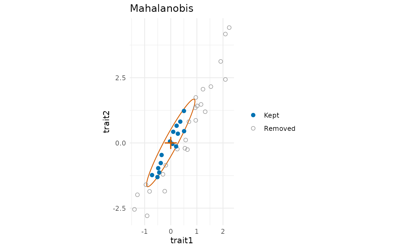
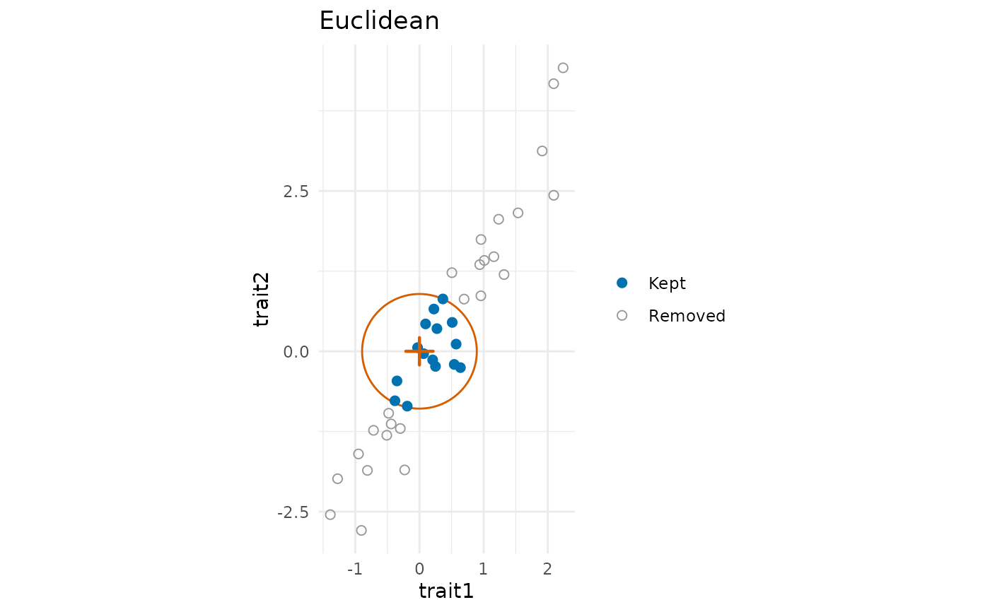
Draws the regional pool in the plane of two traits, with the species kept by
assemble_community() filled and those removed open, in the metric of the assembly:
Arguments
- x
An
mc_assemblyobject fromassemble_community().- traits
The two traits to draw (names or numbers).
- colours
Colours of the species kept and removed, and of the contours.
- species_labels
Should the species be labelled?
- point_size
Size of the species.
- labels, ...
Deprecated:
labelsis nowspecies_labels; graphical arguments of base graphics are no longer used. The aspect ratio is always 1, so that the contours of Euclidean distances are circles.
Details
filtering: the optimum (a cross) and the boundary of the filter, the contour at the distance from the optimum of the farthest species kept (a circle for Euclidean distances, an ellipse for standardized or Mahalanobis distances);
limiting similarity: around each species kept, the contour at half the smallest distance between species kept, so that contours touch but do not overlap;
neutral: the species only.
With more than two traits, the contours are the projections of the ellipsoids on the plane of the two traits, and species that look inside a contour may lie outside it in the other traits.
See also
Other rule-based assembly:
assemble_community()
Examples
set.seed(1)
tr <- treeshapesim::sim_tree_shape(40)
y <- trait_ou(tr, sigma2 = rate_matrix(c(1, 4), correlation = 0.9))
plot_assembly(assemble_community(y, 15, rule = "filtering", optimum = c(0, 0))) +
ggplot2::ggtitle("Euclidean")
 plot_assembly(assemble_community(y, 15, rule = "filtering", optimum = c(0, 0),
distance = "mahalanobis")) +
ggplot2::ggtitle("Mahalanobis")