Simulating lagged series

library(lagprotest)

simulate_lagged_series() generates pairs of multivariate series with a known temporal relationship. It is meant for checking how lagged_protest() behaves in a design like yours before analyzing real data: how often it finds concordance between independent series (Type I error), and how often it detects and locates a true lag (power). This article explains what the function generates and shows a small calibration study.

What the function generates

Each variable of X is a sine wave with period period and amplitude amplitude, plus AR(1) noise with coefficient autocorr and marginal standard deviation noise_sd. All variables share a random phase, offset among variables so that they do not peak at the same time, which gives the series a two-dimensional seasonal trajectory, as in many ecological and physiological data sets.

Y depends on true_lag:

• true_lag = NULL: Y is an independent draw from the same generator, with its own random phase. This is the null hypothesis.
• true_lag = k: Y at time t is a linear map of X at time t − k plus independent AR(1) noise. The map is the identity when X and Y have the same number of variables and a random matrix otherwise. true_lag = 0 is a contemporaneous association, not the absence of one.

sim <- simulate_lagged_series(n_times = 24, n_vars_x = 3, n_vars_y = 3,
                              true_lag = 3, period = 12, autocorr = 0.3,
                              noise_sd = 0.3, seed = 1)
op <- par(mfrow = c(2, 1), mar = c(4, 4, 1, 1))
matplot(sim$X, type = "l", lty = 1, xlab = "Time", ylab = "X")
matplot(sim$Y, type = "l", lty = 1, xlab = "Time", ylab = "Y")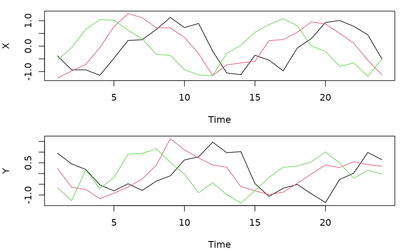

par(op)

Y repeats the seasonal pattern of X three time steps later. The scan recovers the lag:

fit <- lagged_protest(sim$X, sim$Y, lags = 0:6, nperm = 999, seed = 1)
fit$optimal_lag
#> [1] 3
fit$p.global
#> [1] 0.001

Choosing the parameters

The parameters map onto features of a real design:

• n_times: the number of time points you have, for example 12 monthly centroids.
• n_vars_x, n_vars_y: the number of variables (or ordination axes) in each data set. More variables make concordance between independent series more likely by chance, which the permutation null accounts for.
• period: the length of the seasonal cycle in time steps. Setting period = n_times gives one complete cycle; period = 12 with 24 or more monthly samples gives several complete cycles; a period that does not divide n_times gives an incomplete cycle, a case in which the test is not calibrated (see Choosing a permutation scheme).
• amplitude: the strength of the seasonal signal. amplitude = 0 removes it and leaves pure AR(1) series.
• autocorr and noise_sd: the persistence and size of the non-seasonal variation. noise_sd applies both to X and to the noise added to Y. Because Y is a lagged copy of X, including the noise of X, a larger noise_sd weakens the lagged signal less than one might expect; series length has a much stronger effect on power.

A practical way of setting them is to match your data: use your series length and number of variables, estimate the seasonal amplitude and the residual variation from the data, and vary autocorr over a plausible range.

A small calibration study

The function below simulates n_rep pairs, runs lagged_protest() on each, and returns the proportion of replicates in which the global p-value was below α, together with the proportion in which the optimal lag matched the true one. Each replicate gets its own seed, so the study is reproducible.

calibrate <- function(n_rep, true_lag = NULL, n_times = 24, lags = 0:4,
                      nperm = 99, alpha = 0.05, ...) {
  res <- vapply(seq_len(n_rep), function(i) {
    s <- simulate_lagged_series(n_times = n_times, true_lag = true_lag,
                                seed = i, ...)
    f <- lagged_protest(s$X, s$Y, lags = lags, nperm = nperm, seed = i)
    c(reject = f$p.global < alpha,
      lag_found = if (is.null(true_lag)) NA else f$optimal_lag == true_lag)
  }, numeric(2))
  rowMeans(res)
}

Here we use 24 monthly samples spanning two annual cycles, five variables, moderate autocorrelation and lags 0–4. With 100 replicates the estimates are rough (a rate of 0.05 has a 95% interval of about 0.02–0.11); a real study should use 1000 or more replicates and 999 surrogates.

rbind(
  type_I_n24 = calibrate(100, true_lag = NULL, period = 12, autocorr = 0.5,
                         noise_sd = 0.5),
  power_n24 = calibrate(100, true_lag = 2, period = 12, autocorr = 0.5,
                        noise_sd = 0.5),
  power_n12 = calibrate(100, true_lag = 2, n_times = 12, lags = 0:3,
                        period = 12, autocorr = 0.5, noise_sd = 2)
)
#>            reject lag_found
#> type_I_n24   0.03        NA
#> power_n24    1.00      1.00
#> power_n12    0.58      0.95

The first row should be close to 0.05. The second shows that two years of monthly data detect a two-month lag almost always. The third, with a single year of noisier data, shows that the global p-value detects the lag far less often even when the optimal lag is still usually the true one: the lag is easier to locate than to declare significant.

Extending the study

The same function covers other questions by changing its arguments:

• compare schemes by adding permutation = "cyclic" to the call of lagged_protest();
• test the effect of an incomplete seasonal cycle with, for example, n_times = 24, period = 18;
• check robustness to non-seasonal series with amplitude = 0;
• use data sets of different dimension with n_vars_x different from n_vars_y.

For larger studies, run the replicates in parallel (for example with parallel::mclapply() or the future framework); because each replicate has its own seed, results do not depend on how the work is split.